
We have now seen how quantum gates implement unitary transformations on qubits. Intuitively, we should, as in the classical case, now be able to combine these quantum gates into quantum algorithms that perform more complex sequences of manipulations of a quantum state. In this post, we will look at a first example to get an idea how this works. The material in this section is well covered by standard textbooks, like [1] section 3.8 or [2], chapter 6 and chapter 7. In addition, the fundamental structure of quantum algorithm is discussed in the classical papers [3] and [4].
In general, a quantum algorithm can be broken down into several phases. First, we need to initialize the system in a known initial state. Then, we apply a series of transformations, which, as we know, can be described in terms of quantum gates. Finally, we perform a measurement to derive a result.
To illustrate this, let us assume that we are given a more or less arbitrary classical problem that we want to solve using a quantum computer. Formally, this could be a function

mapping binary numbers of length n to binary numbers of length m. We might have an algorithm to calculate this function on a classical computer and are looking for a quantum version of this algorithm.
The first problem we need to solve is that, as we know, quantum algorithms are given by unitary transformations, in particular they are reversible. In the most general setting however, a function f like the one above is not reversible – even if n is equal to m, there is no guarantee that the function is invertible. Fortunately, that can easily be fixed. If we let 

that maps a pair 


Now let us consider a quantum computer that has l qubits, so that its states are given by elements of a Hilbert space of dimension 2l. We can then identify the bit strings of length l, i.e. the elements of 


The transformation Uf is a unitary transformation and, as any unitary transformation, can therefore be decomposed into a sequence of elementary quantum gates. Let us now see how these quantum gates yield an algorithm to calculate f.
Preparing the initial state
First, we need to place our quantum system in some well defined state. For our example, we will use the so-called Hadamard-Walsh transformation to do this. This transformation is defined as the n-fold tensor product of the Hadamard operator H with itself and often denoted by W. Let us see how this operator acts on the state 

Applying the Hadamard operator to each of the n factors individually, we see that this is

Multiplying out this expression, we see that each possible combination of ones and zeros appears exactly once within the sum. In other words, each of the states 

In our case, the state space is a product of n qubits represented by the variable x and m qubits represented by the variable y. As initial state for our quantum algorithm, we will now choose the state that is obtained by applying the Hadamard-Walsh operator W to the first n qubits of the state 

Transformation and measurement
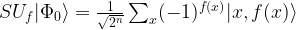
Having defined the initial state, let us now apply the transformation Uf. Using the fact that this transformation is of course linear and the formula for 

It is worth pausing for a moment to take a closer look at this expression. The right hand side of this expression is a superposition of states that encodes the value of f(x) for all possible values of x. Thus, if we can find a way to physically implement quantum devices that are able to
- Initialize an n+m qubit quantum system in a well-known state like
- realize the transformations
and
by a set of quantum gates
we are able to create a state that somehow computes all values f(x) in only one pass of the quantum algorithm.
At the first glance, this sounds like magic. Regardless how big n is, we would be able to calculate all values of f(x) in only one pass of our quantum algorithm! In other words, we would calculate all values of f(x) fully in parallel. This (apparent) feature of quantum computers is often referred to be the term quantum parallelism.
However, there is a twist. Even if we are able to apply a quantum algorithm in order to put our system in a state as above encoding all values of f(x), we still need to be able to extract the actual values of f(x) from that state. Thus, we need to perform a measurement.
If, for instance, we are using a measurement device that corresponds to a projection onto the individual states 

for some value of x. Unfortunately, we cannot tell upfront to which of these vectors we would project. In fact, all these vectors appear with equal amplitude and the probability to obtain each of these vectors is 
But the situation is even worse – once we have executed our measurement, the superposition created by our algorithm is destroyed and the system has collapsed to one of the eigenstates. Thus, if we wanted to perform a large number of measurements in order to obtain f(x) for a given value of x with high probability, we would have to execute our algorithm again for each of the measurements, resulting in a large number of passes. It appears that the advantage of quantum parallelism is lost again….
Fortunately, the situation is not as hopeless as one might think. In many cases, we are not actually interested in all values of f(x). Rather, we are interested in some property of the function f, maybe even in a property that has a simple yes-no answer and can therefore be represented by a single bit. If we find a way to adapt our measuring process by projecting to a different basis or by transforming our state further before measuring, we might be able to get our answer with one measurement only. In the next section, we will look at an algorithm which is in a certain sense the blueprint and inspiration of many other quantum algorithms exploiting this approach.
The Deutsch-Jozsa algorithm
The Deutsch-Jozsa algorithm is a quantum algorithm that tackles the following problem. Suppose we are given a function

We call such a function balanced if the number of times this function takes the value 0 is equal to the number of times this function takes the value 1 (which is obviously only possible if n is even which we will assume).
Now assume that we already know that either f is balanced or f is constant. We want to determine which of these two properties holds. With a classical algorithm, we would have to call f at most n/2 + 1 times, but might as well need this number of invocations for some functions f. In [4], Deutsch and Jozsa presented a quantum algorithm to solve this problem which requires only two applications of the unitary transformation Uf which is the equivalent of applying f in the quantum world, which is generally considered to be the first quantum algorithm that demonstrates a true advantage compared to a classical computation.
To describe the algorithm, we follow the general approach outlined above. We consider a quantum system with n+1 qubits and again denote a basis of the corresponding Hilbert space by 

by applying the Hadamard-Walsh transformation to the state 

Now an additional “smart” operation comes into play. First, we use an operator which is denoted by S in [4] and is defined by

(this is a bit in conflict with our previous notation where we have used the symbol S for the phase shift operator, but let us again this for now to stay aligned with the notation in [4]). When we apply the operator S to our state, we obtain
Finally, we apply the inverse of Uf, which is actually Uf itself, as a straightforward calculation on basis vectors using the definition of Uf shows. Thus we end up with the state

Let us now compute the overlap, i.e. scalar product, of this state with the state 

we obtain

Now suppose that we perform a measurement corresponding to the projection onto the subspace spanned by 
How would we actually perform such a measurement, assuming that we can measure the individual qubits of our quantum computer? To perform a measurement corresponding to the projection onto 

and we see that

We can now repeat our previous argument to link the structure of f to the outcome of a measurement. In fact, if f is constant, the scalar product is one and our final state will be a multiple of 
Now measurement in the standard basis corresponds to successive measurement of all individual qubits. Thus in the first case, all bits will be measured as zero with certainty, and in the second case, at least one bit will be measures as one with certainty. Hence we arrive at the following form of the algorithm.
- Prepare the quantum system in the initial state
- Apply the Hadamard-Walsh transformation to the first n qubits
- Apply Uf, then apply the phase shift operator f and then apply Uf once more
- Finally apply the Hadamard-Walsh transformation once more to the first n qubits and measure all qubits
- If the measurement yields zero for all qubits, the function f is constant, otherwise the function f is balanced
This version of the algorithm, which is essentially the version presented in the original paper [4], uses two invocations of Uf. Later, a slighly more efficient version of the algorithm was developed ([5]) that only requires one application of Uf. From a theoretical point of view, it is less important whether we need one or two “calls” to Uf – the crucial point is that quantum parallelism makes the number of invocations constant, independent of the value of n. However, from a practical point of view, i.e. when it comes to an implementation on a real quantum computer, being able to reduce the number of involved qubits and gates is of course essential. We briefly sketch the required circuit which we will also see again when we discuss other algorithms.
Given a function f, this circuit will create the state 


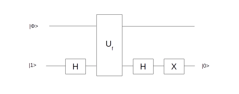
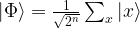
Let us quickly check that the circuit is doing what we want. It starts with the superposition across all states x that we denote by
Then we add an ancilla qubit initialized to

We now let Uf act on this state. If f(x) is zero for some value of x, this transformation maps 


and consequently

which is the same as

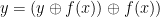
Now applying the Hadamard operator once more to the ancilla qubit followed by the negation operator X transforms the ancilla qubit to 
The Deutsch-Jozsa algorithm is widely acknowledged as the first real quantum algorithm that leverages the potential of a quantum computer and achieves a real improvement compared to classical hardware, while still yielding a deterministic result despite the stochastic nature of quantum systems. Of course, the problem solved by the algorithm is mainly of academical interest. In the next few posts, we will move on to study other algorithms that have been developed in the sequel that are more relevant for actual applications.
References
1. G. Benenti, G. Casati, G. Strini, Principles of Quantum Computation and Information, Volume 1, World Scientific
2. E. Rieffel, W. Polak, Quantum computing – a gentle introduction, MIT Press
3. D. Deutsch, Quantum Theory, the Church-Turing principle and the Universal Quantum Computer, Proceedings of the Royal Society of London A. Vol. 400, No. 1818 (1985), pp. 97-117
4. D. Deutsch, R. Jozsa, Rapid Solution of Problems by Quantum Computation, Proceedings of the Royal Society of London A, Vol. 439, No. 1907 (1992), pp. 553-558
5. R. Cleve, A. Ekert, C. Macchiavello, M. Mosca, Quantum algorithms revisited, arXiv:quant-ph/9708016


 , a unitary transformation is of course given by a unitary 2×2 matrix.
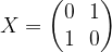
 and is therefore sometimes called the bit-flip or negation. Its eigenvalues are 1 and -1, with a pair of orthogonal and normed eigenvectors given by


 and
and  , and, as
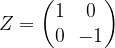
  , vice versa. Similarly, the phase operator
 for this. In this basis, the CNOT gate is given by the following 4 x 4 matrix:
 and
and  to itself and swaps the vectors
  and
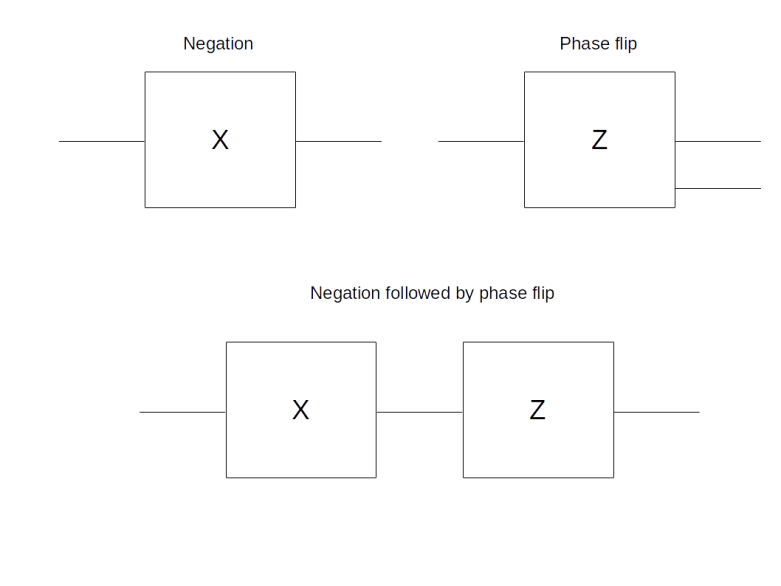
and  . Thus, expressed in terms of bits, it negates the second bit if the first bit is ON and keeps the second bit as it is if the first bit is OFF. Thus, the first bit can be thought of as a control bit that controls whether the second bit – the target bit – is toggled or not, and this is where the name comes from, CNOT being the abbreviation for “controlled NOT”. Graphically, the CNOT gate is represented by a small circle on the control bit and an encircled plus sign on the target bit (this is the convention used in
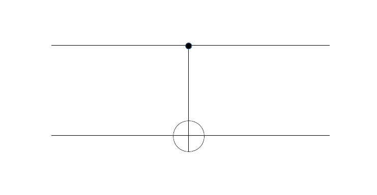
 . This state can as well be written as

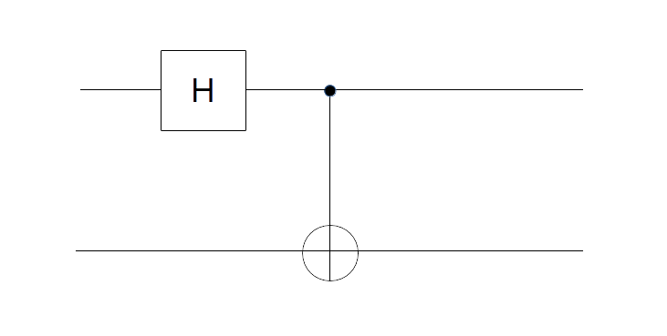
 . We read the circuit from the left to the right and the top to the bottom. Thus, the first part of the circuit acts with H on the first qubit and with the identity on the second qubit. It therefore maps the state

 to
to  . Thus the entire circuit maps the vector
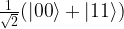
 to
to  , and it is well known that any such function can be expressed as a combination of gates from a small set of standard gates called universal gates. In fact, it is even true that one gate is sufficient – the NAND gate. It is natural to ask whether the same is true for quantum gates. More precisely, can we find a finite set of unitary transformations such that any n-qubit unitary transformation can be composed from them using a few standard operations like the tensor product?
 phase gate.

 as eigenvectors, with eigenvalues 0 and 1, i.e. it is given by the matrix

 , we can form the tensor product

 and
and 
 and
and 

 and
and  , we obtain
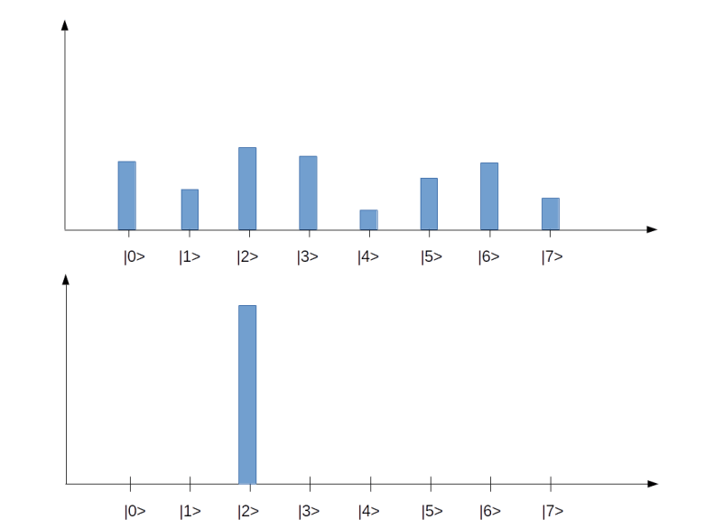
 . In our example, we have eight basis states, corresponding to a quantum system with 3 qubits. The bar represents the amplitude, i.e. the number
  in the superposition above (of course this is only a very incomplete representation, as it represents the amplitudes as real numbers, whereas in reality they are complex numbers). The upper state in the diagram represents a superposition for which all of the amplitudes are different from zero. The second diagram represents a state in which all but one amplitude is zero, i.e. a state that is equivalent to one of the basis vectors (
 in this case). These states correspond to the eight states of a corresponding classical system with three bits, whereas all states with more than one bar are true superpositions which have no direct equivalent in the classical case. We will later see how similar diagrams can be used to visualize the inner workings of simple quantum algorithms.
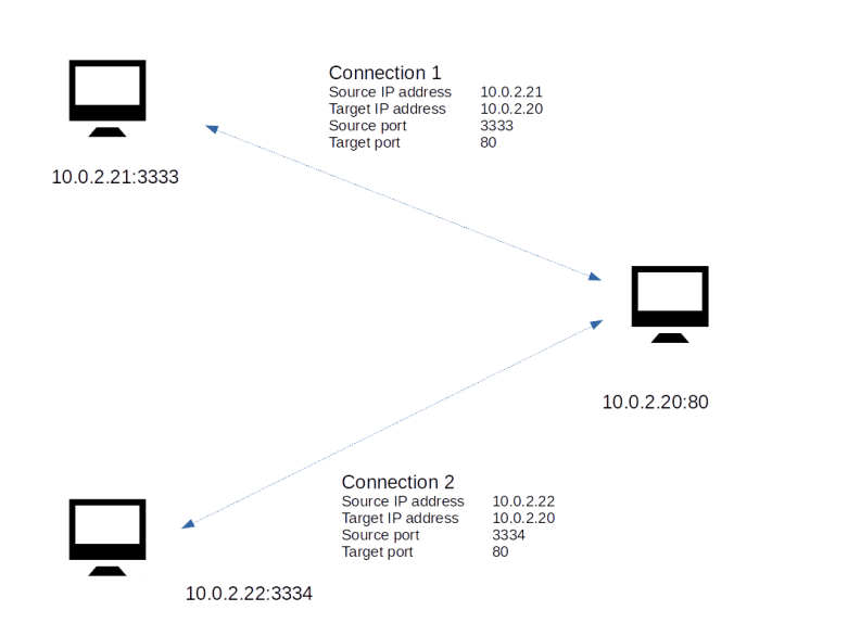


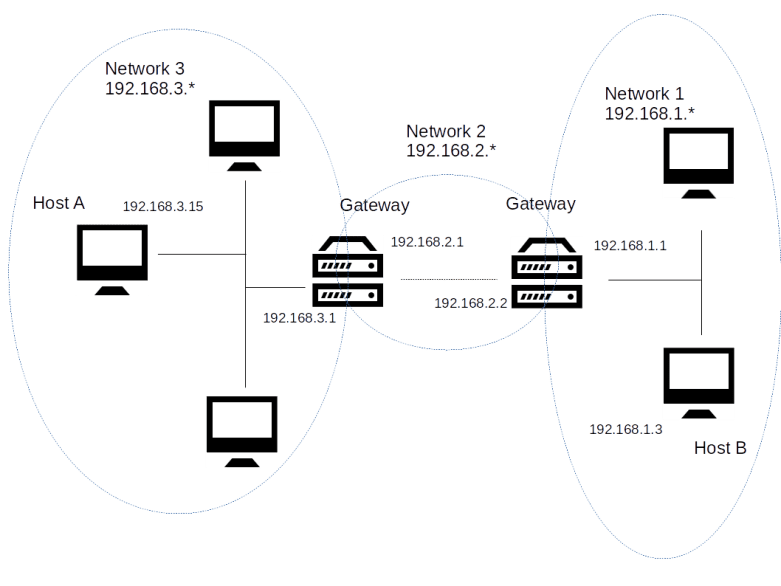


 Both networks are connected by a third network, indicated by the dashed line. This network can use any other link layer technology. Each network contains a dedicated host called the gateway that connects the network to this third network.