In my previous post on quantum error correction, we have looked at the toric code which is designed for a rather theoretical case – a grid of qubits on a torus. In reality, qubits are more likely to be arranged in a planar geometry. Luckily, a version of the toric codes that works well in a planar geometry exists – the surface code.
Planar codes and their stabilizers
Recall that the starting point for the toric code was a lattice L with periodic boundary conditions so that the geometry of the lattice becomes toroidal, which gave us a four-dimensional code space.
If we want to use this code in planar setting, it is clear that we somehow have to modify the boundary conditions. What happens if we simply drop it? A short calculation using a bit of algebraic topology shows that in this case, the code space collapses to a one-dimensional code space which is not enough to hold a logical qubit. So we need some a more sophisticated boundary condition. The solution found in [1] is to use two types of boundaries.
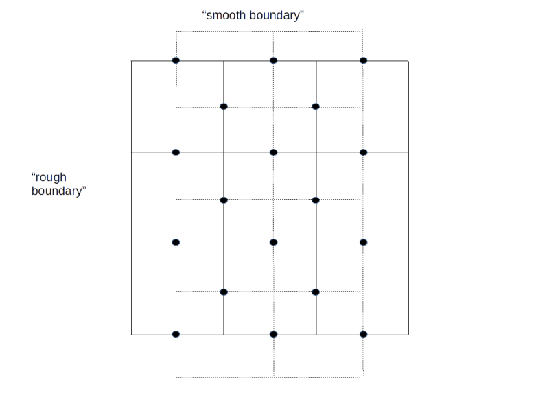
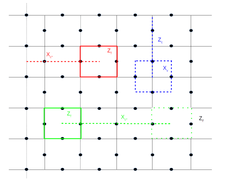
Look at the diagram above. The solid lines form a lattice L with two types of boundary – a “smooth” boundary at the top and the bottom and a “rough boundary” left and right (ignore the dashed lines for a moment, we will explain their meaning in a second). We again place qubits on the edges of the lattice, but for the boundary, we only place qubits (again indicated by black dots) on the edges which are part of the smooth boundary.
As for the case of a toric code, we can again create a second lattice called the dual lattice whose vertices are the center points of the faces of L and whose edges are perpendicular to the edges of L. This dual lattice is indicated by the dashed lines in our diagram. Again, some edges of the dual lattice carry qubits and others do not, so we have a smooth and a rough boundary as well (note that the smooth boundary of L gives raise to the rough boundary of the dual lattice and vice versa).
Again a path along the edges, i.e. a set of edges, is an element of a group, the group of one chains. If we only allow the edges that are not part of the rough boundary, i.e. the edges that carry qubits, we obtain a subgroup which is known to topologists as the group of one chains relative to the rough boundary – again I will strive to keep this post free from too much algebraic topology and refer the reader to my notes for more details and a more precise description.
As for the toric code, every such relative one-chain c gives raise to a operators Xc and Zc, obtained by letting X respectively Z act on any qubit crossed by the chain. Similarly, a co-chain is a path in the dual lattice, i.e. a path perpendicular to the edges of the lattice L.
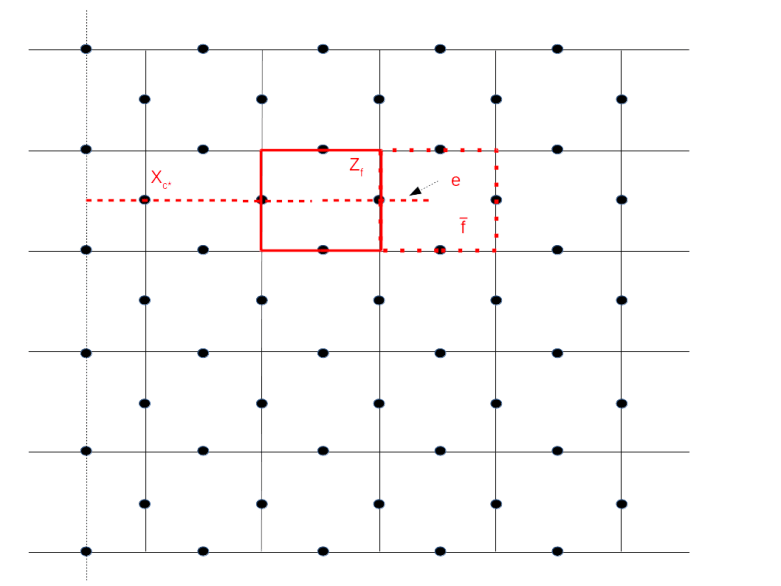
In the literature, the lattice and its dual are typically visualized differently, namely with all edges that do not carry qubits removed, as in the following diagram.
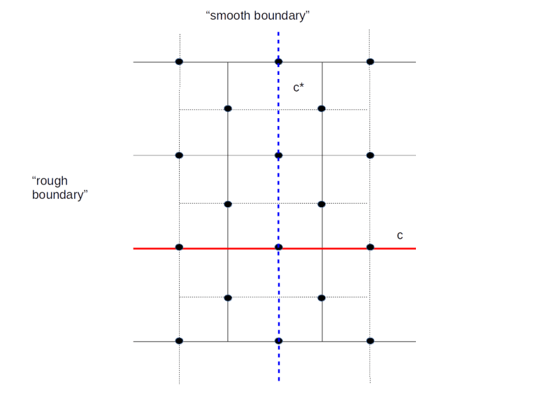
Here we have removed the rough boundary at the left and right of the lattice and the same for the dual lattice. The red line is a relative one chain. Note that this one-chain is “open-ended”. Its boundary would be in the (removed) rough boundary. In the relative version of the chain complex, its boundary is zero, hence this is the equivalent to a closed loop in the toric geometry. Similarly, the blue line represents a co-chain, i.e. a chain in the dual lattice, which has zero boundary in the dual lattice.
We can now proceed as for the toric code. For each vertex v, there is a vertex operator Xv, which is the product of the Pauli X operators acting on the qubits sitting on the edges touching the vertex (which are four qubits in the interior of the lattice and three qubits if the vertex is sitting on the smooth boundary). For each face f, we again have a face operator Zf, acting as a Pauli Z operator on the four qubits sitting on the boundary edges of the face – again, if the face is located at the rough boundary, there are only three operators. These operators again commute with each other and create an abelian subgroup S. The code space TS created by this group, i.e. the space of all states left invariant by all face operators and all vertex operators, now turns out to be two-dimensional and is thus encoding one logical qubit. The code obtained in this way is called the surface code.
Again, there are logical Pauli operators. In fact, these are the operators created by the chains marked in the diagram above – the Z operator Zc associated with the one chain c and the X operator Xc* associated with the co-chain c*. The fact that these operators commute with each operator in S is related to their boundaries being zero (in the sense described above, i.e. the are open-ended) and the fact that they anti-commute is expressed geometrically by the fact that they intersect exactly once.
Thus we obtain a logical qubit and logical Pauli operators that act on this qubit. What about measurements? As for the toric code, we can measure our (data) bits located at the edges by adding measurement qubits. To measure a face operator Zf, we can place an additional measurement qubit in the center of the face and use this qubit as an ancilla in our measurement circuit below.
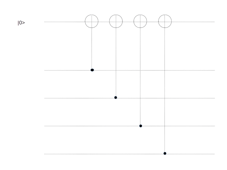
Similarly, to measure the vertex operator Xv for a vertex v, we place an additional measurement qubit at the vertex and use a similar circuit to transfer the result of the measurement into this qubit, as we did it for the toric code. The only difference to the case of a toric code is again that if a vertex or face is adjacent to only three qubits as it is located close to the boundary, we only include those qubits in our measurement. We therefore obtain the following arrangement of qubits, were black dots are data qubits, white dots are ancilla qubits used for the measurements and a letter X or Z indicates the action of a Pauli operator (this is, up to a switch of black and white, the graphical representation of a surface code used in [2]).
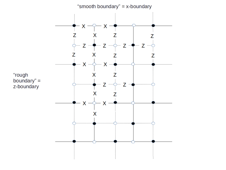
For instance, a white dot surrounded by Z’s indicates a face and the corresponding face operator Zf, together with the black data qubits on which the face operator acts. At the same time, the white dot is the location of a measurement qubit used to measure Zf. Similarly, a white dot surrounded by X’s indicates both a vertex operator and a data qubit to measure the vertex operator.
Of qubits and holes
So far we have seen how the surface code can be used to encode a single logical qubit in a whole array of physical qubits. In practice, however, we need more than one qubit. We could of course try to arrange the planar surfaces in a stack, with qubits on each plane interacting with the qubits above and below, and then use some variant of quantum teleportation to establish connectivity between the logical qubits. However, there is a different way – we can realize more than one logical qubit on one array of physical qubits (this is only one option – as of today, there are many different approaches built upon similar ideas, like color codes or lattice surgery – see [5] and [6] for a discussion of some alternatives).
The idea is simple. We have obtained our code space as the intersection of the subspaces given by constraints, where each face operator and each vertex operator add one (linear) constraint. To obtain a larger code space, all we have to do is to drop a few of these constraints again!
To understand how this works, we first have to understand how the surface code is usually used in practice ([2]). We first put the system into an initial, potentially unknown state. We then perform a series of measurements of all stabilizers. This will force the state into a simultaneous eigenstate of all the stabilizer operators.
Now, the eigenvalues will typically not all be one. We therefore have to apply corrections to move our state into the code space (or we could as well keep track of the error syndrome and perform the corrections in software when we measure) – this is exactly the same process as if we had found errors during the later computation. In other words, we do a first round of error correction.
We now start our quantum algorithm. After each step of the algorithm, we perform another round of measurements of the stabilizers to detect any errors that might have occurred. Again, we could now correct the errors, or alternatively keep track of them as well and correct the final measurements if needed. In this way, a computation with a surface code is essentially a periodic measurement of all stabilizers in repeating cycles followed by an (actual or virtual) error correction, and logical operations executed between any two subsequent cycles.
Now let us see what happens when we modify our code by removing a face operator Zf from the set of stabilizers. Thus we perform some initial cycles to put the system into a ground state  (here and in the sequel, we assume that errors are actually corrected and not just detected to simplify our calculations) on which all stabilizers act trivially, and starting with the next round of measurements, we exclude a Zf operator from the measurements.
Of course, this will enlarge the code space. Specifically, let us take a look at the upper left corner of the figure above. Here we have marked a face f and an operator Xc* coming from a string connecting this face with the rough boundary. Then the boundary of c* consists of one point in the dual lattice (the center of f), and hence every face operator commutes with Xc*, except Zf which anti-commutes. If we now define our code space to be the space fixed by all the vertex operators Xv and all face operators except Zf, then Xc* and Zf map that code space to itself. As c* intersects the boundary of f in one point, Zf and Xc* anti-commute and therefore define a set of logical Pauli operators, acting on the code space. Thus we have constructed a logical qubit!
Intuitively, removing the face operator Zf from the set of stabilizers corresponds to poking a “hole” into the surface, i.e. removing the face f and the data qubit in it. But of course we do not change the physical layout of our device at all – all we do is changing the code space and the set of logical Pauli operators. Our original code space, by the way, still exists, but we will tacitly ignore it and work with our new logical qubit.
This construction has a nice physical interpretation in terms of the particle picture that we have introduced in the post on the toric code. Suppose we create a pair of quasi-particles, supported on f and a second face close to the rough boundary. We have seen that we can move these particles by acting with edge operators Xe on them. Thus, we can move the second face on which the particle lives across the rough boundary and now obtain a particle supported on one face only. This is exactly the configuration which is obtained by acting with the logical Pauli X operator of our newly created logical qubit on the ground state, i.e. these logical qubits correspond to pairs of particles where one particle has been “pushed off” the surface!
As usual, this construction has a counterpart in the dual lattice, as shown on the right of of our diagram. The configuration marked in blue consists of a vertex operator Xv and a string c connecting that vertex to the smooth boundary. We can now remove Xv from the stabilizer, and obtain a pair of logical operators Xv and Zc. This type of logical qubit is called a single X-cut in [2], whereas the first type of qubit considered is a single Z-cut – other authors use the term defects for these logical qubits.
This technique allows us in theory to encode a large number of logical qubits in one surface. However, in practice, the restriction that we need to reach the boundary from each of the faces and vertices that we switch off is restricting our layout options a bit. Fortunately, it turns out that this is not even necessary.
In fact, coming back to the analogy of the quasi-particles, nobody forces us to move the second particle off the surface. To see this, consider the configuration marked in green in the lower part of the diagram above. Here we have removed two stabilizers from the code, the face operator Zf corresponding to the face on the left hand side, and the face operator Zf’ corresponding to the face on the right hand side. This will enlarge our code space by a space of dimension four. However, we now gracefully ignore half of that space and instead work with the space spanned by the Pauli operators Zf and Xc*.
A logical qubit obtained by this construction is called a double Z-cut. Of course, we can again repeat this construction in the dual lattice and obtain a double X-cut (these cuts are also for vegetarians…).
Let’s do the twist – moving and braiding qubits
Again, it is time to recap what we have done so far. We have seen that we can create logical qubits by removing face and vertex operators from the set of stabilizers. We have also seen that we can identify logical Pauli X and Z operators acting on these qubits. We can than, of course, also realize a logical Y as the product ZX. What about other gates? And specifically, what about multi-qubit gates?
It turns out that multi-qubit gates can be realized by moving logical qubits around the surface. To make this term a bit more precise, take a look at the following diagram.
Here we consider a logical qubit described by the Pauli operators Xc* and Zf, i.e the face operator Zf has been removed from the set of stabilizers. Adjacent to the face f, there is a face that we denote by  . By removing
  (and adding Zf again to the set of stabilizers), we would obtain a different code space – we can think of this different code space as a deformation of the code space given by removing Zf.
We want to describe a process that starts with a state in the code space given by Zf and ends with a state in the code space given by . To do this, we manipulate the original state in several steps. First, we measure the Pauli X operator Xe for the physical qubit sitting on the edge e of the dual lattice that connects the centre of f with that of – this is the qubit on which both and Zf act. Let us assume for a moment that the outcome of this measurement is one. Next, we do another measurement – this time we measure Zf. This will force the system into an eigenstate of Zf. Let us assume again that the outcome of this measurement is plus one, so that the system is now in the new code space obtained by removing instead of Zf from the stabilizer.
This procedure gives us a mechanism to transform a state in the original code space into a state in the new code space. It is not difficult to see (again I refer to my notes for all the details) that this leaves the logical meaning of the state untouched, i.e. this transformation maps a logical one in the old codespace to a logical one in the new code space and the same for a logical zero (in fact, it turns out that we need to modify the Pauli operators a bit for this to work).
Of course we cannot directly compare the states before and after the transformation as they live in different code spaces. That, however, changes if we move a logical state around like this along a closed loop. Then we will obtain a new state which is living in the original code space and can compare it directly to the original state, as in the diagram below.
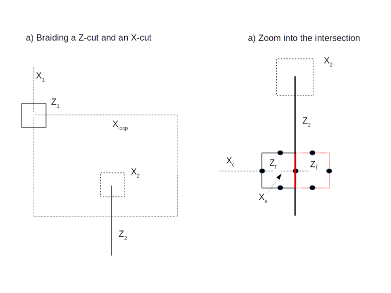
This diagram shows an example where we move a logical qubit generated by a Z-cut once around a logical qubit generated by an X-cut. If we hit upon the intersection between the loop and the X-cut, we pick up an additional transformation. This is a bit like a coordinate transformation – while we move along the loop, we constantly have to adjust our coordinate system, i.e. the logical Pauli operators, to preserve the logical meaning of the qubit. When we reach the initial position, we now have two coordinate system that we can compare, and we find that we have picked up a non-trivial transformation related to the fact that we cannot contract the loop without passing the hole in the surface creating our logical qubit. If you go through all the transformations carefully (or read my notes where I have tried to work out all the details – it is easy to get confused at this point), you will find that the transformation we pick up constitutes a CNOT gate between the two involved qubits! Thus a CNOT can be realized by moving one logical qubit around the second logical qubit once. This is often visualized by a two-strand braid, as illustrated below.
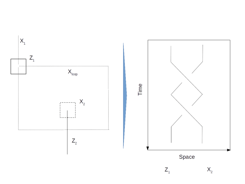
We have also seen that the transformation given by such a braiding operation is governed by terms like intersection numbers and contracting loop, i.e. the transformation is topological in nature – a slightly deformed braid or path gives the same result. Therefore this operation has a certain natural protection against faults, it is topologically protected. Unfortunately, the surface code does not allow a representation of a universal set of quantum gates by braids – doing this requires the use of a more sophisticated physical equivalent called non-abelian anyons. For the surface code, for instance, the T gate cannot be represented by topological operations and needs to be implemented using a technique called gate teleportation.
We will not go into details on this, but try to quickly describe the basic idea which is based on the observation that the circuit
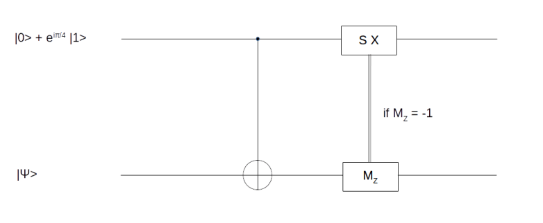
can be used to realize the T gate.
How does this circuit work? The upper qubit is an ancilla qubit that is initialized with the specific state

by a process called magic state distillation (see [2] for details). Now a short calculation shows that after applying the CNOT gate, the combined system of both qubits will be in the state

Thus we have successfully transferred the state  into the first qubit (this is why this and similar circuits are called gate teleportation circuits), but still have a superposition. To remove this superposition, we nown perform a measurement MZ on the second qubit. If the outcome of this measurement is one, the first qubit will be in the state
  and we are done. If not, i.e. if the measurement results in minus one, then the above formula shows that the resulting state in the first qubit will be
  . Now one can easily verify that

and

so that if we apply the sequence SX to the first qubit conditioned on the outcome of the measurement, as indicated in our circuit diagram, the result will in both cases be .
By now, our discussion should have made it clear that the surface codes create a significant overhead. To illustrate this, the appendix of [2] contains an estimation of the number of physical qubits needed to implement Shor’s factoring algorithm for a 2048 bit RSA key. Still, most operations on a surface code are topologically protected, which makes surface codes rather robust. Therefore surface codes remain a promising technology to implement universal fault-tolerant quantum computation, and are one of the most active areas of current research in applied quantum computing.
References
1. S. Bravyi, A. Kitaev, Quantum codes on a lattice with boundary, arXiv:quant-ph/9811052
2. A.G. Fowler, M. Mariantoni, J.M. Martinis, A.N. Cleland, Surface codes: Towards practical large-scale quantum computation, arXiv:1208.0928v2
3. A.G. Fowler, A.M. Stephens, P. Groszkowski, High threshold universal quantum computation on the surface code, arXiv:0803.0272
4. E. Dennis, A. Kitaev, A. Landahl, J. Preskill, Topological quantum memory, arXiv:quant-ph/0110143
5. T.J. Yoder, I.H. Kim, The surface code with a twist, Quantum Vol. 1, 2017 (available online)
6. A. Javadi-Abhari et. al., Optimized Surface Code Communication in Superconducting Quantum Computers, arXiv:1708.09283

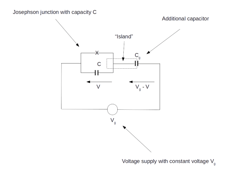
![H = E_C[N - N_g] - E_0 \cos \delta](https://s0.wp.com/latex.php?latex=H+%3D+E_C%5BN+-+N_g%5D+-+E_0+%5Ccos+%5Cdelta++&bg=FFFFFF&fg=000&s=1&c=20201002)

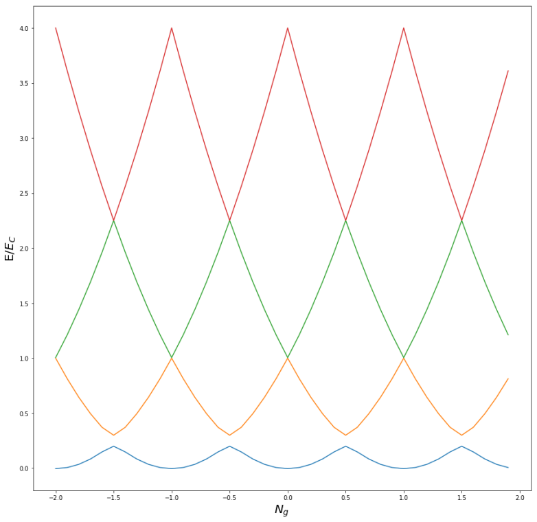
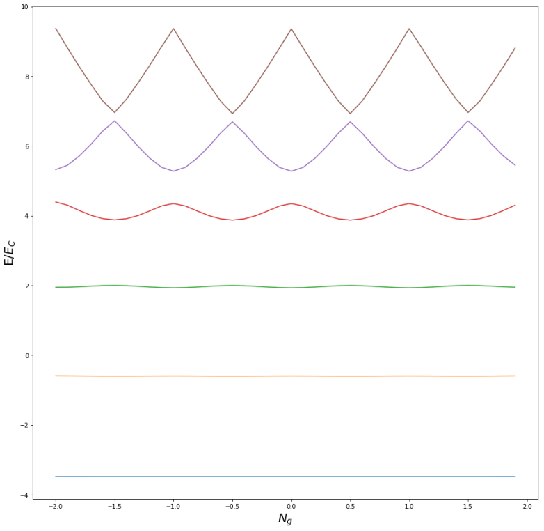


 is a state localized around the left minimum of the potential and
  is a state centered around the right minimum, whereas the first excited state is a linear combination proportional to
 in an interpretation as a qubit – and our first excited state
  are superpositions of these two states.


 .
.


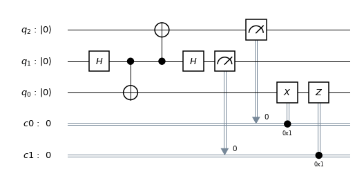
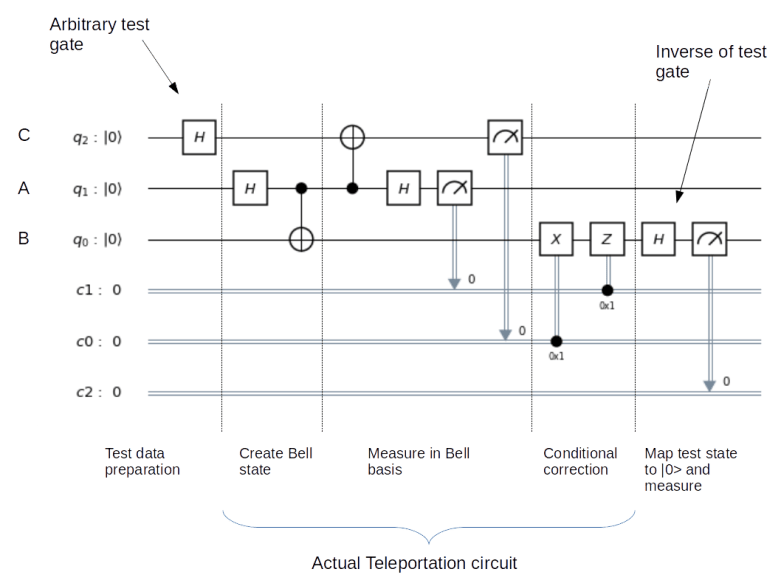
 , stored in some sort of quantum device, which could be a superconducting qubit, a trapped ion, a polarized photon or any other physical implementation of a qubit. Bob is operating a similar device. The task is to create a quantum state in Bob’s device which is identical to the state stored in Alice device.
 (we use the lower index to denote the qubit in which the state lives). We also assume that Alice is able to perform arbitrary measurements and operations on A and C, and that B similarly controls qubit B.
![|\beta_{00}^{AB} \rangle = \frac{1}{\sqrt{2}} \big[ |0\rangle _A |0 \rangle _B+ |1\rangle_A |1 \rangle_B) \big]](https://s0.wp.com/latex.php?latex=%7C%5Cbeta_%7B00%7D%5E%7BAB%7D+%5Crangle+%3D+%5Cfrac%7B1%7D%7B%5Csqrt%7B2%7D%7D+%5Cbig%5B+%7C0%5Crangle+_A+%7C0+%5Crangle+_B%2B+%7C1%5Crangle_A+%7C1+%5Crangle_B%29+%5Cbig%5D++&bg=FFFFFF&fg=000&s=1&c=20201002)
 indicates the two qubits in which the Bell state vector lives. This is the common state mentioned above, and it can obviously be prepared upfront, without having the state
 ![|\beta_{00}^{AB} \rangle |\psi\rangle_C = \frac{1}{\sqrt{2}} \big[ a |000 \rangle + a |110 \rangle + b |001\rangle + b |111 \rangle \big]](https://s0.wp.com/latex.php?latex=%7C%5Cbeta_%7B00%7D%5E%7BAB%7D+%5Crangle+%7C%5Cpsi%5Crangle_C+%3D+%5Cfrac%7B1%7D%7B%5Csqrt%7B2%7D%7D+%5Cbig%5B+a+%7C000+%5Crangle+%2B+a+%7C110+%5Crangle+%2B+b+%7C001%5Crangle+%2B+b+%7C111+%5Crangle+%5Cbig%5D++&bg=FFFFFF&fg=000&s=1&c=20201002)
![\frac{1}{\sqrt{2}} \big[ a |000 \rangle + a |101 \rangle + b |010\rangle + b |111 \rangle \big]](https://s0.wp.com/latex.php?latex=%5Cfrac%7B1%7D%7B%5Csqrt%7B2%7D%7D+%5Cbig%5B+a+%7C000+%5Crangle+%2B+a+%7C101+%5Crangle+%2B+b+%7C010%5Crangle+%2B+b+%7C111+%5Crangle+%5Cbig%5D++&bg=FFFFFF&fg=000&s=1&c=20201002)
 . Using the table above, we can express our state in this basis. This will give us four terms that contain a and four terms that contain b. The terms that contain a are
![\frac{a}{2} \big[ |\beta^{AC}_{00}\rangle |0 \rangle + |\beta^{AC}_{10}\rangle |0 \rangle + |\beta^{AC}_{01}\rangle |1 \rangle - |\beta^{AC}_{11} \rangle |1 \rangle \big]](https://s0.wp.com/latex.php?latex=%5Cfrac%7Ba%7D%7B2%7D+%5Cbig%5B+%7C%5Cbeta%5E%7BAC%7D_%7B00%7D%5Crangle+%7C0+%5Crangle+%2B+%7C%5Cbeta%5E%7BAC%7D_%7B10%7D%5Crangle+%7C0+%5Crangle+%2B+%7C%5Cbeta%5E%7BAC%7D_%7B01%7D%5Crangle+%7C1+%5Crangle+-+%7C%5Cbeta%5E%7BAC%7D_%7B11%7D+%5Crangle+%7C1+%5Crangle+%5Cbig%5D++&bg=FFFFFF&fg=000&s=1&c=20201002)
![\frac{b}{2} \big[ |\beta^{AC}_{01}\rangle |0 \rangle + |\beta^{AC}_{11}\rangle |0 \rangle + |\beta^{AC}_{00}\rangle |1 \rangle - |\beta^{AC}_{10} \rangle |1 \rangle \big]](https://s0.wp.com/latex.php?latex=%5Cfrac%7Bb%7D%7B2%7D+%5Cbig%5B+%7C%5Cbeta%5E%7BAC%7D_%7B01%7D%5Crangle+%7C0+%5Crangle+%2B+%7C%5Cbeta%5E%7BAC%7D_%7B11%7D%5Crangle+%7C0+%5Crangle+%2B+%7C%5Cbeta%5E%7BAC%7D_%7B00%7D%5Crangle+%7C1+%5Crangle+-+%7C%5Cbeta%5E%7BAC%7D_%7B10%7D+%5Crangle+%7C1+%5Crangle+%5Cbig%5D++&bg=FFFFFF&fg=000&s=1&c=20201002)
 . Thus there are four different possible outcomes of this measurement, which we can read off from the expansion in terms of the Bell basis above.


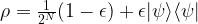
 – of them are in a pure state. The second term in this expression is often called the deviation and denoted by
  .
.
 . Similarly, one can show that if A is an observable, described by a hermitian matrix (which, for technical reasons, we assume to be traceless), then the expectation value of A evaluated on


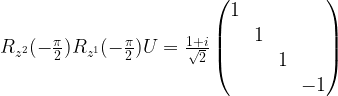
 . The matrix on the right hand side of this equation represents a two-qubit transformation known as the controlled phase gate. This gate corresponds to applying a phase gate to the second qubit, conditional on the state of the first qubit.


 .
.
 and the spin operator
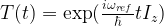
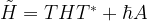
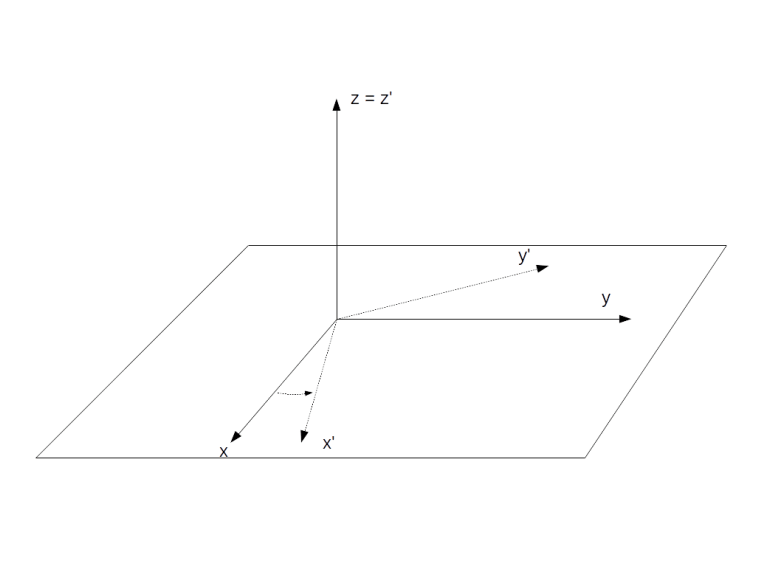
 . Geometrically, this is a rotation around the z-axis by the angle
  . Using the formula above and the fact that T commutes with the original Hamiltonian, we find that the transformed Hamiltonian is

 , we place ourselves in a frame of reference rotating with the same frequency around the z-axis. In this rotating frame, the state vector will be constant, corresponding to the fact that the new Hamiltonian vanishes. If we choose a reference frequency different from the Larmor frequency, we will observe a precession with the frequency
  .
.
![H = \omega I_z + \omega_{nut} [I_x \cos (\omega_{ref}t + \Phi_p) + I_y \sin (\omega_{ref}t + \Phi_p) ]](https://s0.wp.com/latex.php?latex=H+%3D+%5Comega+I_z+%2B+%5Comega_%7Bnut%7D+%5BI_x+%5Ccos+%28%5Comega_%7Bref%7Dt+%2B+%5CPhi_p%29+%2B+I_y+%5Csin+%28%5Comega_%7Bref%7Dt+%2B+%5CPhi_p%29+%5D++&bg=FFFFFF&fg=000&s=1&c=20201002)
![\tilde{H} = \omega_{nut} [I_x \cos \Phi_p + I_y \sin \Phi_p ]](https://s0.wp.com/latex.php?latex=%5Ctilde%7BH%7D+%3D+%5Comega_%7Bnut%7D+%5BI_x+%5Ccos+%5CPhi_p+%2B+I_y+%5Csin+%5CPhi_p+%5D++&bg=FFFFFF&fg=000&s=1&c=20201002)
 . The time evolution of this density matrix is governed by the Liouville-von Neumann equation
![i\hbar \frac{d}{dt} \rho = [H,\rho]](https://s0.wp.com/latex.php?latex=i%5Chbar+%5Cfrac%7Bd%7D%7Bdt%7D+%5Crho+%3D+%5BH%2C%5Crho%5D++&bg=FFFFFF&fg=000&s=1&c=20201002)
 is a traceless hermitian matrix. Any such matrix can be expressed as a linear combination of the Pauli matrices with real coefficients. Consequently, we can write


 (the reason for this notation will become apparent in a second) and a unit vector n.
![[a\cdot I, b \cdot I] = i \hbar (a \times b) \cdot I](https://s0.wp.com/latex.php?latex=%5Ba%5Ccdot+I%2C+b+%5Ccdot+I%5D+%3D+i+%5Chbar+%28a+%5Ctimes+b%29+%5Ccdot+I++&bg=FFFFFF&fg=000&s=1&c=20201002)
![\dot{f} = - \omega_{eff} [f \times n]](https://s0.wp.com/latex.php?latex=%5Cdot%7Bf%7D+%3D+-+%5Comega_%7Beff%7D+%5Bf+%5Ctimes+n%5D++&bg=FFFFFF&fg=000&s=1&c=20201002)
 . Therefore, according to the density matrix formalism, the expectation value of the x-component of the magnetic moment
  is
is
 and use the fact that the trace of a product of two different Pauli matrices is zero, we find that the only term that contributes to the trace is the term fx, i.e.


 , we can write this as


 , this changes. We have already seen that in the rotating frame, this pulse adds an additional term

 . If, for instance, we choose
  , the vector f – and thus the magnetic moment – will slowly rotate around the x-axis. If we turn off the pulse after a time

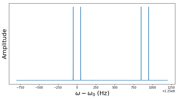
 of the first nucleus and the reference frequency, so that the value zero corresponds to

 is the usual Pauli Z-operator, i.e. the Hamiltonian is simply a multiple of the Pauli Z operator. Consequently, the time evolution operator is
 . Thus, on the Bloch sphere, the time evolution is a rotation around the z-axis with frequency
 , then the nuclear spin will flip into a direction perpendicular to the z-axis.

 . The elements of this group are simply binary linear combinations of edges, i.e. subsets of all edges. Addition in this group is given by joining the subsets, while dropping elements that appear twice. As there is one qubit sitting on every edge, every chain c, i.e. every subset of edges, will yield an operator that we call Xc and which is simply given by applying the Pauli X operator to each of the qubits sitting on an edge appearing in c. Similarly, one can define an operator Zc for evey chain c by combining the Pauli Z operators for the qubits touched by c.
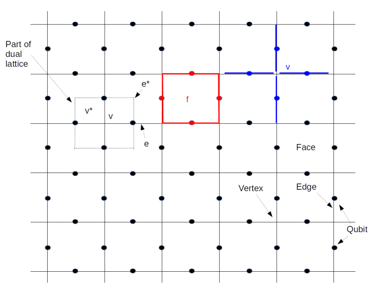
 . As described above, we can associate an operator
  to this one chain, which is simply given by letting a Pauli Z operator act on each of the qubits sitting on the red edges. This operator is called the face operator associated with the face f and denoted by Zf
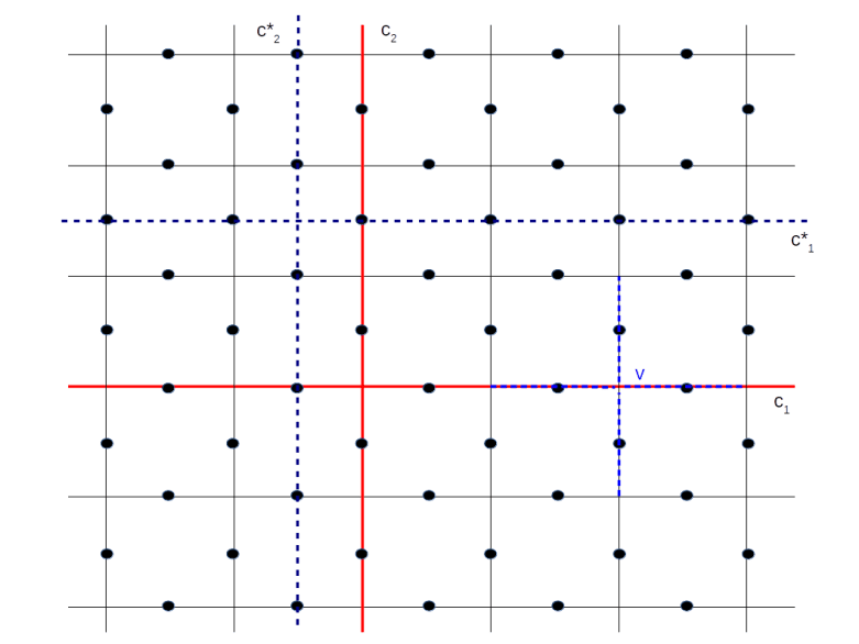
 to be the state which is left invariant by these two operators.
 . Each of these vectors is an eigenstate of all face and vertex operators, and we denote the corresponding eigenvalues by xvi and zfi. Clearly,
  is then an eigenvector of H with eigenvalue
 into eigenstates of the Hamiltonian, the above discussion shows that the eigenvalue has increased by four. Thus errors correspond to excited states, and the operators Zc are creation operators that create excited states that are in a certain sense localized at the vertices of the lattice. It is tempting and common to therefore call these excitations quasi-particles, similar to the phonons in a crystal lattice.
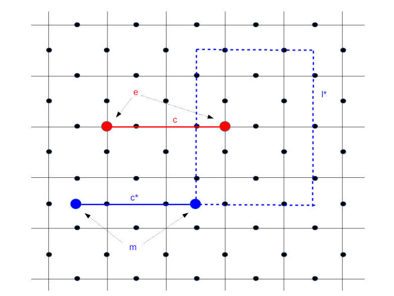
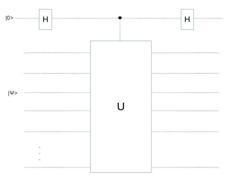

![\frac{1}{\sqrt{2}} \big[ |0 \rangle |\psi \rangle + |1 \rangle |\psi \rangle \big]](https://s0.wp.com/latex.php?latex=%5Cfrac%7B1%7D%7B%5Csqrt%7B2%7D%7D+%5Cbig%5B+%7C0+%5Crangle+%7C%5Cpsi+%5Crangle++%2B+%7C1+%5Crangle+%7C%5Cpsi+%5Crangle+++%5Cbig%5D++&bg=FFFFFF&fg=000&s=1&c=20201002)
![\frac{1}{\sqrt{2}} \big[ |0 \rangle \otimes |\psi \rangle + |1 \rangle \otimes U |\psi \rangle \big]](https://s0.wp.com/latex.php?latex=%5Cfrac%7B1%7D%7B%5Csqrt%7B2%7D%7D+%5Cbig%5B+%7C0+%5Crangle+%5Cotimes+%7C%5Cpsi+%5Crangle++%2B++%7C1+%5Crangle+%5Cotimes+U+%7C%5Cpsi+%5Crangle++%5Cbig%5D++&bg=FFFFFF&fg=000&s=1&c=20201002)
 is an eigenstate with eigenvalue plus one and
  an eigenstate with eigenvalue minus one. Plugging this into the above equation and applying the final Hadamard operator shows that the final outcome of the circuit will be
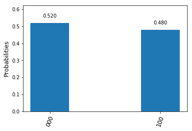
 or
or  , with probabilities
  and
and  . The remaining qubits end up in the state
  , i.e. in an eigenstate. Thus applying this circuitry and measuring the ancilla has the same implications as measuring the operator U and yields the same information.
 operators, i.e. inversion operators. Therefore a controlled-Xv circuit is nothing but a sequence of controlled inversions, i.e. CNOT gates. Thus we can measure a vertex operator using the following circuit.
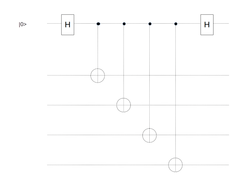
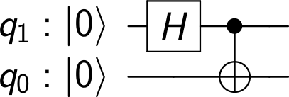
 , we can construct such a circuit as follows. In the first time step, apply a Hadamard to both the ancilla and all target qubits. Then apply CNOT operators to all target qubits, controlled by the ancilla, and then apply Hadamard operators again. Now, it is well known that conjugating the CNOT with Hadamard gates switches the roles of target qubits and control qubits. This gives us the circuit displayed below.
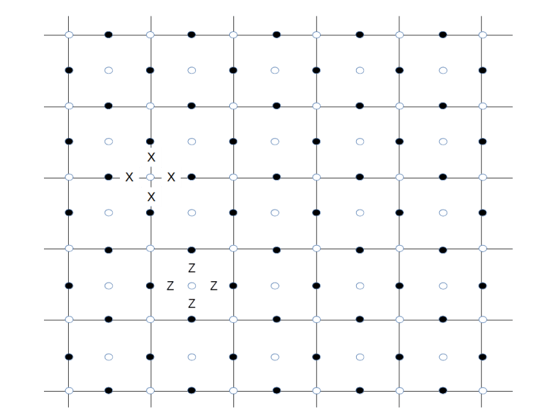
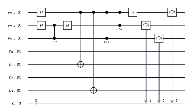
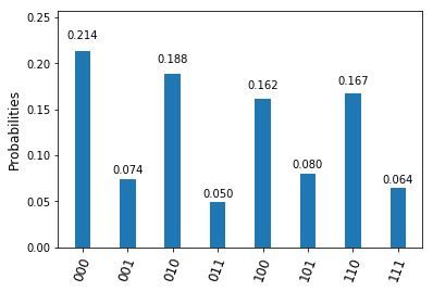
 and to which we apply a sequence of controlled multiplications by powers of a, and a working register, in which we do a quantum Fourier transform in the second step. The primary register needs to hold M=15, so we need four qubits there. For the working register, we use three qubits, which is the smallest possible choice, to keep the number of gates small.
 . Thus we only need to implement a unitary transformation which conditionally maps the state
  . In binary notation, eleven is 1011, and we therefore simply need to conditionally flip qubits 3 and 1. We also need a Pauli X gate in the primary register to build the initial state
  and Hadamard gates in the working register to create the initial superposition. Thus the first part of our circuit looks as follows.


 , and we can again implement this by two conditional bit flips, i.e. two CNOT gates.


