April 2020 – LeftAsExercise

OpenStack Cinder – creating and using volumes

In the previous post, we have installed Cinder and described its high level architecture. Today, we will look at a few uses cases (creating and attaching volumes) in detail, go through the code and see how Cinder interacts with external technologies like iSCSI and LVM.

Creating a volume

Let us first try to understand what happens when a volume is created, for instance because a user submit the corresponding API request via the OpenStack CLI, using v3 of the API.

In the architecture overview, we have mentioned that the Cinder API server is run by Apache. To understand how this request is processed, it therefore makes sense to start at the Apache2 configuration in /etc/apache2/conf-available/cinder-wsgi.conf. Here, we find a reference to the script cinder-wsgi which in turn shows up in the setup.cfg file distributed with Cinder. Following the link in this file, we find that the WSGI server is initialized by initialize_application which in turn uses the Oslo service library to create an application from a PasteDeploy configuration.

Browsing the PasteDeploy config that is distributed with Cinder, we find that, as we have seen it before, it defines several authorization strategies. We use the Keystone strategy, and in this pipeline, the last element points to the factory method cinder.api.v3.router.APIRouter.factory, implemented here. This class implements a routing mechanism, which translates our PUT request into a call to VolumeController.create.

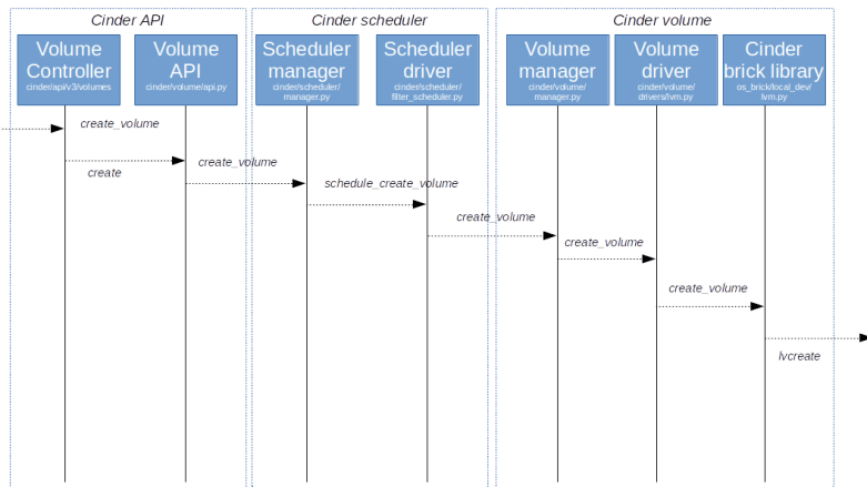
So far, this flow looks familiar and we have seen this before – there is a WSGI application acting as an API endpoint, which routes requests to various controller. Now the Cinder specific processing starts, and the Controller, after performing some transformations and validations, invokes cinder.volumes.API().create()

This method now uses a device which we can find at several points in OpenStack when it comes to managing processes consisting of several steps – the OpenStack Taskflow library. This library provides flows that can be built from tasks, can be run using a flow engine and can be stopped and reverted in a controlled manner. In Cinder, various processes are modeled as flows. In our case, the flow is built by this method and consists of several tasks, which will deduct the volume size from the quota, create a database object for the volume and commit the changed quota. If everything succeeds, we now delegate to the scheduler for further processing by triggering a RPC call via RabbitMQ.

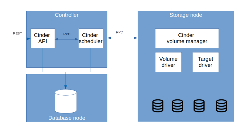
The entry point into the scheduler, which is running as an independent process, is the method create_volume of the corresponding manager object cinder.scheduler.SchedulerManager. Here, we create another flow and run it. This flow does again do some validation and then calls a scheduler driver, which, as so often in OpenStack, is a pluggable module that carries out the actual scheduling. In our case, this is the filter scheduler. After the actual scheduling is complete, the driver now sends an RPC call to the selected node which is received by the volume manager, more precisely by its method create_volume.

This again creates a flow, which will include a task that does the actual volume creation (CreateVolumeFromSpecTask). Here, the actual work is delegated to a volume driver. In our setup, our driver is the LVM driver (cinder.volume.drivers.LVMVolumeDriver). We first look at its _init_ method. Here we determine the target_helper from the configuration and create the corresponding target driver. During initialization, the manager will also call the method check_for_setup_error which, among other things, creates an object which represents the volume group that Cinder manages and which is an instance of cinder.brick.local_dev.LVM. When the method create_volume of the volume driver is called, it will essentially delegate the call to this class. In its create_volume method, we now finally see that the LVM command lvcreate is called which creates the actual logical volume.

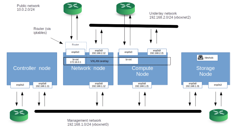
Let us try to find the traces of all this in our setup. For that purpose, re-start the setup from the previous setup, and, if you have not yet done so, create a volume of size 1 (GB).

git clone https://github.com/christianb93/openstack-labs
cd openstack-labs/Lab13
vagrant up
ansible-playbook -i hosts.ini site.yaml
ansible-playbook -i hosts.ini demo.yaml
vagrant ssh network
source demo-openrc
openstack volume create \
  --size 1 \
  demo-volume

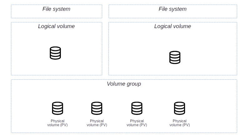
Now log out of the network node, log into the storage node and run sudo lvs. You should see two volumes, both on top of the volume group cinder-volumes, as in the sample output below.

  LV                                          VG             Attr       LSize Pool                Origin Data%  Meta%  Move Log Cpy%Sync Convert
  cinder-volumes-pool                         cinder-volumes twi-aotz-- 4.75g                            0.00   10.64                           
  volume-5eae9e4b-6a28-41a2-a983-e435ec23ce46 cinder-volumes Vwi-a-tz-- 1.00g cinder-volumes-pool        0.00

We see that there is a new logical volume, whose name is the prefix volume-, followed by the UUID of the volume that we have just created. This is a so-called thin volume, meaning that LVM does not allocate extends when the logical volume is created, but maintains a pool of available extends and allocates extends from this pool only when data is actually written. This is a sort of over-commitment of storage, as it allows us to create volumes which have a size much larger than the actually physically available size.

Attaching a volume

At this point, we have created a virtual storage volume which is living on the storage node. In order to be usable for an instance, we now have to attach the volume to an instance. Before trying this out, let us again see how this request will flow through the source code.

Typically, attaching a volume is done by a call to the Nova API. Nova will then in turn call the Cinder API where the calls will be processed by the Cinder attachment controller. Actually, during the process of attaching a volume to an instance, Nova will invoke the Cinder API three times (not counting read-only requests). First, it will use a POST request to ask the controller to create the attachment, then it will use a PUT request to update the attachment by providing so-called connector information and finally, it will use another POST request to call the complete method to signal that the process of attaching the volume is complete.

Let us start to understand the first request. Here, Nova only provides the UUID of the volume and the UUID of the instance to be connected. This request will be served by the create method of the attachment controller. After some preparations, the controller will then invoke the method attachment_create of the volume manager API. At this point, no connector information is available yet, so all this method does is to create a reservation by storing the attachment in the database.

Now the second call from Nova comes in. At this point, Nova will have collected the connector information, which is the IP address of the compute node, the iSCSI initiator name, the mount point and some additional information. Just in case you want to link this back into the Nova code: the connector data is assembled here (where we can also see that the IP address used is taken from the configuration item my_block_storage_ip in the Nova configuration), and the update call to the Cinder API which we are currently discussing is made here.

A typical connector information could look as follows.

{'connector': 
  {'platform': 'x86_64', 
   'os_type': 'linux', 
   'ip': '192.168.1.21', 
   'host': 'compute1', 
   'multipath': False, 
   'initiator': 'iqn.1993-08.org.debian:01:a41db8382266', 
   'do_local_attach': False, 
   'system uuid': '54F9944F-66C9-411E-9989-84AB5CEE6B18', 
   'mountpoint': '/dev/vdc'}
}

The update call will again reach the volume manager API which will look up the volume and forward the request via RPC to the volume manager on the storage node where the storage is located. The result – the connection information – is then returned to the callee, i.e. in our case the Nova driver, which then connects to the device using a volume driver and eventually submits the third call to Cinder to signal completion.

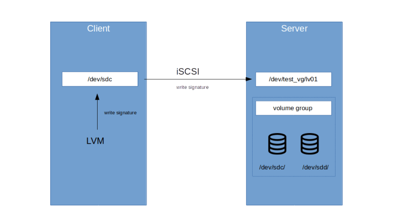
But let us continue to investigate the call chain for the update call first. The volume manager on the storage node now performs several steps. First, it calls the responsible Cinder volume driver (which, in our case, is the LVM driver) to create the export, i.e. to activate the logical volume and to use a target driver to initiate the actual export. In our case, the target driver is the iSCSI driver, and export here simply means that an iSCSI target is created on the storage driver (and a CHAP secret is returned).

Back in the volume manager, the manager next calls the method initialize_connection of the driver which is simply passed through to the target driver and assembles the connection information, i.e. the target and portal information. Finally, the manager makes a call to the method attach_volume of the volume driver, but this method is empty for the LVM driver. At this point, the database record is updated and the connection info is returned.

Nova is now able to finalize the attachment by using the Open-iSCSI helper to establish the connection to the target using iscsiadmin from the Open-iSCSI package. When all this succeeds, Nova will eventually call Cinder a third time, this time invoking the complete method of the attachment controller. This method will update the attachment and the volume in the database, and the entire process is complete.

Let us now try to identify some of the objects created during this process in our lab setup. For that purpose, first log into the networking node and attach the volume that we have just created to our instance.

source demo-openrc
openstack server \
  add volume \
  demo-instance-3 \
  demo-volume

Now log out off the network node and log into the compute node. Here, we first use iscsiadm to display all open iSCSI sessions.

sudo iscsiadm -m session -P 3

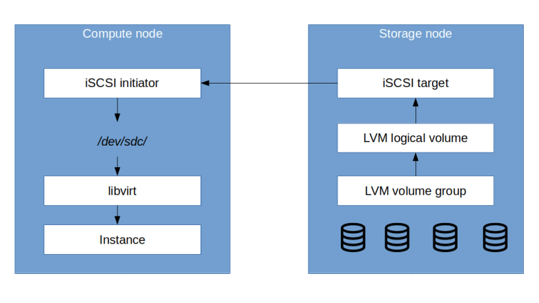
Here you can see that we have an open session connected to the iSCSI target that Cinder has created for this volume, and you can see that this volume is mapped to a block device like /dev/sdc on the compute node. Note that there is actually one target for each volume, so that a dedicated CHAP secret can be used for every logical volume.

Now let us try to locate this block device in the configuration of our KVM/QEMU guest. For this purpose, we first use the OpenStack API to determine the UUID of the instance and then the virsh manager to display this instance.

source demo-openrc
uuid=$(openstack server show \
  demo-instance-3 \
  -c id -f value)
sudo virsh domblklist $uuid

We now see that the instance has two devices attached to it. The first device is mapped to /dev/vda inside the instance and is the root device. This device is a flat file that Nova has created and placed on the compute host, i.e. it is an ephemeral device which gets lost if the instance is destroyed, the host goes down or the instance is migrated to a different machine. The second device is our device /dev/sdc which is pointing via iSCSI to the virtual device on the storage node.

There are many other functions of Cinder that we have not yet touched upon. You can, for instance, create volumes from existing images, in which case Glance comes into play, or Cinder can use the snapshot functionality of LVM to create and manage snapshots. It is also possible to configure Cinder such that is uses mirrored LVM devices (with a local mirror, though), and of course there are many other volume drivers apart from LVM. Going through all this would be a separate series, but I hope that I could at least provide some entry points into code and documentation so that you can explore all this if you want.

OpenStack Cinder – architecture and installation

Having looked at the foundations of the storage technology that Cinder uses in the previous posts, we are now ready to explore the basic architecture of Cinder and install Cinder in our playground.

Cinder architecture

Essentially, Cinder consists of three main components which are running as independent processes and typically on different nodes.

First, there is the Cinder API server cinder-api. This is a WSGI-server running inside of Apache2. As the name suggests, cinder-api is responsible for accepting and processing REST API requests from users and other components of OpenStack and typically runs on a controller node.

Then, there is cinder-volume, the Cinder volume manager. This component is running on each node to which storage is attached (“storage node”) and is resonsible for managing this storage, i.e. preparing, maintaining and deleting virtual volumes and exporting these volumes so that they can be used by a compute node. And finally, Cinder comes with its own scheduler, which directs requests to create a virtual volume to an appropriate storage node.

Of course, Cinder also has its own database and communicates with other components of OpenStack, for example with Keystone to authenticate requests and with Glance to be able to create volumes from images.

Cinder van use a variety of different storage backends, ranging from LVM managing local storage directly attached to a storage node over other standards like NFS and open source solutions like Ceph to vendor-specific drivers like Dell, Huawei, NetApp or Oracle – see the official support matrix for a full list. This is achieved by moving low-level access to the actual volumes into a volume driver. Similarly, Cinder uses various technologies to connect the virtual volumes to the compute node on which an instance that wants to use it is running, using a so-called target driver.

To better understand how Cinder operates, let us take a look at one specific use case – creating a volume and attaching to an instance. We will go in more detail on this and similar use cases in the next post, but what essentially happens is the following:

A user (for instance an administrator) sends a request to the Cinder API server to create a logical volume
The API server asks the scheduler to determine a storage node with sufficient capacity
The request is forwarded to the volume manager on the target node
The volume manager uses a volume driver to create a logical volume. With the default settings, this will be LVM, for which a volume group and underlying physical volumes have been created during installation. LVM will thzen create a new logical volume
Next, the administrator attaches the volume to an instance using another API request
Now, the target driver is invoked which sets up an iSCSI target on the storage node and a LUN pointing to the logical volume
The storage node informs the compute node about the parameters (portal IP and port, target name) that are needed to access this target
The Nova compute agent on the compute node invokes an iSCSI initiator which maps the iSCSI target into the local file system
Finally, the Nova compute agent asks the virtual machine driver (libvirt in our case) to attach this locally mapped device to the instance

Installation steps

After this short summary of the high-level architecture of Cinder, let us move and try to understand how the installation process looks like. Again, the installation follows the standard pattern that we have now seen so many times.

Create a database for Cinder and prepare a database user
Add user, services and endpoints in Keystone
Install the Cinder packages on the controller and the storage nodes
Modify the configuration files as needed

In addition to these standard steps, there are a few points specific for Cinder. First, as sketched above, Cinder uses LVM to manage virtual volumes on the storage nodes. We therefore need to perform a basic setup of LVM on each storage node, i.e. we need to create physical volumes and a volume group. Second, every compute node will need to act as iSCSI initiator and therefore needs a valid iSCSI initiator name. The Ubuntu distribution that we use already contains the Open-iSCSI package, which maintains an initiator name in the file /etc/iscsi/initiatorname.iscsi. However, as this name is supposed to be unique, it is not set in the Ubuntu Vagrant image and we need to do this once during the installation by running the script /lib/open-iscsi/startup-checks.sh as root.

There is an additional point that we need to observe which is also not mentioned in the official installation guide for the Stein release. When installing Cinder, you have to define which network interface Cinder will use for the iSCSI traffic. In production, you would probably want to use a separate storage network, but for our setup, we use the management network. According to the installation guide, it should be sufficient to set the configuration item my_ip, but in reality, this did not work for me and I had to set the item target_ip_address on the storage nodes.

Lab13: running and testing the Cinder installation

Time to try this out and set up a lab for that. The first thing we need to do is to modify our Vagrantfile to add a storage node. In order to reduce memory consumption a bit, we instead move from having two computes to one compute node only, so that our new setup looks as follows.

As mentioned above, we will not use a dedicated storage network, but send the iSCSI traffic over the management network so that our network setup remains essentially unchanged. To bring up this scenario and to run the Cinder installation plus a demo setup do the following.

git clone https://github.com/christianb93/openstack-labs
cd openstack-labs/Lab13
vagrant up
ansible-playbook -i hosts.ini site.yaml
ansible-playbook -i hosts.ini demo.yaml

When all this completes, we can run some tests. First, verify that all storage nodes are up and running. For that purpose, log into the controller node and use the OpenStack CLI to retrieve a list of all recognized storage nodes.

vagrant ssh controller
source admin-openrc
openstack volume service list

The output that you get should look similar to the sample output below.

+------------------+-------------+------+---------+-------+----------------------------+
| Binary           | Host        | Zone | Status  | State | Updated At                 |
+------------------+-------------+------+---------+-------+----------------------------+
| cinder-scheduler | controller  | nova | enabled | up    | 2020-01-01T14:03:14.000000 |
| cinder-volume    | storage@lvm | nova | enabled | up    | 2020-01-01T14:03:14.000000 |
+------------------+-------------+------+---------+-------+----------------------------+

We see that there are two services that have been detected. First, there is the Cinder scheduler running on the controller node, and then, there is the Cinder volume manager on the storage node. Both are “up”, which is promising.

Next, let us try to create a volume and attach it to one of our test instances, say demo-instance-3. For this to work, you need to be on the network node (as we will have to establish connectivity to the instance).

vagrant ssh network
source demo-openrc
openstack volume create \
  --size=1 \
  demo-volume
openstack server add volume \
  demo-instance-3 \
  demo-volume
openstack server show demo-instance-3
openstack server ssh \
  --identity demo-key \
  --login cirros \
  --private demo-instance-3

You should now be inside the instance. When you run lsblk, you should find a new block device /dev/vdb being added. So our installation seems to work!

Having a working testbed, we are now ready to dive a little deeper into the inner workings of Cinder. In the next post, we will try to understand some of the common use cases in a bit more detail.

OpenStack Cinder foundations – building logical volumes and snapshots with LVM

When you want to build a volume service for a cloud platform, you need to find a way to quickly create and remove block devices on your compute nodes. We could of course use loopback devices for this, but this is slow, as every operation goes through the file system. A logical volume manager might be a better alternative. Today, we will investigate the logical volume manager that Cinder actually uses – Linux LVM2.

The Linux logical volume manager – some basic terms

In this section, we will briefly explain some of the key concepts of the Linux logical volume manager (LVM2). First, there are of course physical devices. These are ordinary block devices that the LVM will completely manage, or partitions on block devices. Technically, even though these devices are called physical devices in this context, these devices can themselves be virtual devices, which happens for instance if you run LVM on top of a software RAID. Logically,
the physical devices are divided further into physical extents. An extent the smallest unit of storage that LVM manages.

On the second layer, LVM now bundles one or several physical devices into a volume group. On top of that volume group, you can now create logical devices. These logical devices can be thought of as being divided into logical extents. LVM maps these logical extents to physical extents of the underlying volume group. Thus, a logical device is essentially a collection of physical extents of the underlying volume group which are presented to a user as a logical block device. On top of these logical volumes, you can then create file systems as usual.

Why would you want to do this? One obvious advantage is again based on the idea of pooling. A logical volume essentially pools the storage capacity of the underlying physical devices and LVM can dynamically assign space to logical devices. If a logical device starts to fill up while other logical devices are still mostly empty, an administrator can simply reallocate capacity between the logical devices without having to change the physical configuration of the system.

Another use case is virtualization. Given that there is sufficiently storage in your logical volume group, you can dynamically create new logical devices with a simple command, which can for instance be used to automatically provision volumes for cloud instances – this is how Cinder leverages the LVM as we will see later on.

Looking at this, you might be reminded of a RAID controller which also manages physical devices and presents their capacity as virtual RAID volumes. It is important to understand that LVM is not (primarily) a RAID manager. In fact, newer versions of LVM also offer RAID functionality (more on this below), but this it not its primary purpose.

Another useful functionality that LVM offers is a snapshot. When you create a snapshot, LVM will not simply create a physical copy. Instead, it will start to mark blocks which are changed after the snapshot has been taken as changed and only copy those blocks to a different location. This makes using the snapshot functionality very efficient.

Lab12: installing and using LVM

Let us now try to see how LVM works in practice. First, we need a machine with a couple of unused block devices. As it is unlikely that you have some spare disks lying around under your desk, we will again use a virtual machine for that purpose. So bring up our test machine and log into it using the following commands (assuming that you have gone through the basic setup steps in the the first post in this series).

git clone https://github.com/christianb93/openstack-labs
cd openstack-labs/Lab12
vagrant up
vagrant ssh box

When you now run lsblk inside the machine, you should see two additional devices /dev/sdc and /dev/sdd which are both unmounted and have a capacity of 5 GB each.

As a first step, let us now prepare these physical volumes for use with LVM. This is done using the pvcreate utility. WARNING: if you accidentally run this outside of the VM, it will render the device unusable!

sudo pvcreate /dev/sdc
sudo pvcreate /dev/sdd

What is this command actually doing? To understand this, let us first use pvscan to print a list of all physical volumes on the system which LVM knows.

sudo pvscan -u

You will see a list of two volumes, and after each volume, LVM will print a UUID for this volume. Now let us see what LVM has actually written on the volume.

sudo dd if=/dev/sdc \
  bs=1024 \
  count=10 \
  | hexdump -C

In the output, you will see that LVM has written some sort of signature onto the device, containing some binary information and the UUID of the device. In fact, this is how LVM stores state and is able to recognize a volume even if it has been moved to a different point in /dev.

Now we can build our first volume group. For that purpose, we use the command vgcreate and specify the name of the volume group and a list of physical devices that the volume group should contain.

sudo vgcreate test_vg /dev/sdc /dev/sdd

If you now repeat the dump above, you will see that LVM has again written some additional data on the device, we find the name of the newly created volume group and even a JSON representation of the physical volumes in the volume group.

Let us now print out a bit more information on the system using the lvm shell. So run

sudo lvm

to start the shell and then type fullreport to get a description of the current configuration. It is instructive to play a bit with the shell, use help to get a list of available commands and exit to exit the shell when you are done.

Finally, it is now time to create a few logical volumes. Our entire volume group has 10 GB available. We will create three logical volumes which in total consume 6 GB.

for i in {1..3}; do
  sudo lvcreate \
    --size 2G \
    test_vg \
    --type linear \
   --name lv0$i
done
sudo lvscan

The last command will print a list of all logical volumes on the system and should display the three logical volumes that we have just created. If you now again create a full report using lvm, you will find these three devices and a table that indicates how the logical extends are distributed across the various physical devices.

Behind the scenes, LVM uses the Linux device mapper kernel module, and in fact, each device that we create is displayed in the /dev tree at three different points. First, LVM exposes the logical volumes at a location built according to the scheme

/dev/volume group name/logical volume name

In our example, the first volume, for instance, is located at /dev/test_vg/lv01. This, however, is only a link to the device /dev/dm-0, indicating that it is created by the device mapper. Finally, a second link is created in /dev/mapper.

The LVM metadata daemon

We have said above that LVM stores its state on the physical devices. This, however, is only a part of the story, as it would imply that whenever we use one of the tools introduced above, we have to scan all devices, which is slow and might interfere with other read or write access to the device.

For that reason, LVM comes with a metadata daemon, running as lvmetad in the background as a systemctl service. This daemon maintains a cache of the LVM metadata that a command like lvscan will typically use (you can see this if you try to run such a command as non-root, which will cause an error message while the tool is trying to connect to the daemon via a Unix domain socket).

The metadata daemon is also involved when devices are added (hotplug), removed, or changed. If, for example, a physical volume comes up, a Linux kernel mechanism known as udev informs LVM about this event, and when a volume group is complete, all logical volumes based on it are automatically activated (see the comment on use_lvmetad in the configuration file /etc/lvm/lvm.conf).

It is interesting to take a look at the udev ruleset that LVM creates for this purpose (you will find these rules in the LVM-related files in /lib/udev/rules.d, in my distribution, these are the files with the numbers 56 and 69). In the rules file 69-lvm-metad.rules, for instance, you will find a rule that invokes (via systemd dependencies) a pvscan every time a physical device is added which will update the cache maintained by the metadata daemon (see also this man-page for a bit more background on the various options that you have to activate logical LVM devices at boot-time).

However, there is one problem with this type of scan that should be mentioned. Suppose, in our scenario, someone exports our logical device /dev/test_vg/lv01 using a block device level tool like iSCSI. A client then consumes the device and it appears inside the file system of the client as, say, /dev/sdc. On the client, an administrator now decides to also use LVM and sets up this device as a physical volume.

LVM on the client will now write a signature into /dev/sdc. This write will go through the iSCSI connection and the signature will be written to /dev/test_vg/lv01 on the server. If now LVM on the server scans the devices for signatures the next time, this signature will also appear on the server, and LVM will be confused and believe that a new physical device has been added.

To avoid this sort of issues, the LVM configuration file /etc/lvm/lvm.conf contains an option which allow us to add a filter to the scan, so that only devices which are matching that filter are scanned for PV signatures. We will need this when we later install Cinder which uses LVM to create logical volumes for virtual machines on the fly.

LVM snapshots

Let us now explore a very useful feature of LVM – efficiently creating COW (copy-on-write) snapshots.

The idea behind a copy-on-write snapshot is easily explained. Suppose you have a logical volume that contains, say, 100 extends. You now want to create a snapshot, i.e. a copy of that volume at a given point in time. The naive approach would be to go through all extents and to create an exact copy for each of them. This, however, has two major disadvantages – it is very time consuming and it requires a lot of additional disk space.

When using copy-on-write, you would proceed differently. First, you would create a list of all extents. Then, you would start to monitor write activities on the original volume. As soon as an extent is about to be changed, you would mark it as changed and create a copy of that extent to preserve its content. For those extents, however, that have not yet changed since the snapshot has been created, you would not create a copy, but refer to the original content when someone tries to read from the snapshot, similar to a file system link.

Thus when a read is done on the snapshot, you would first check your list whether the extent has been changed. If yes, the copied extent is used. If no, the read is redirected to the original extent. This procedure is very fast, as we do not have to copy around all the data at the time when the snapshot is created, and uses space efficiently, as the capacity needed for the snapshot does not depend on the total size of the original volume, but on the volume of change.

Let us try this out. For this exercise, we will use the logical volume /dev/test_vg/lv01 that we have created earlier. First, use fdisk to create a partition on this volume, then create a file system and a mount point and mount this volume under /mnt/lv/ . Note that – which confused me quite a bit when trying this – the device belonging to the partition will NOT show in in /dev/test_vg, but in /dev/mapper/, i.e. the path to the partition that you have to use with mkfs is /dev/mapper/test_vg-lv01p1. Then create a file in in the mounted directory.

(echo n; echo p; echo 1; echo ; echo ; echo w)\
  | sudo fdisk /dev/test_vg/lv01
sudo partprobe /dev/test_vg/lv01
sudo mkfs -t ext4 /dev/mapper/test_vg-lv01p1
sudo mkdir -p /mnt/lv
sudo mount /dev/mapper/test_vg-lv01p1 /mnt/lv
echo "1" |  sudo tee /mnt/lv/test
sudo sync

Note that we need one execution of partprobe to force the kernel to read the partition table on the logical device which will create the device node for the partition. We also sync the filesystem to make sure that the write goes through to the block device level.

Next, we will create a snapshot. This done using the lvcreate command as follows.

sudo lvcreate \
  --snapshot \
  --name snap01 \
  --size 128M \
  --permission r \
  test_vg/lv01

There are two things that should be noted here. First, we explicitly specify a size of the snapshot which is much smaller than the original volume. At a later point in time, when a lot of data has been written, we might have to extend the volume manually, or we can make use of LVMs auto-extension feature for snapshots (see the comments for the parameter snapshot_autoextend_threshold in /etc/lvm/lvm.conf and the man page of dmeventd which needs to be running to make this work for details). Second, we ask LVM to create a read-only snapshot – LVM can also create read-write snapshots, which in fact is the default, but we will not need this here.

If you now run lvs to get a list of all logical volumes, you will see that a new snapshot volume has been created which is linked (via the “origin” field) to the original volume. Let us now mount the snapshot as well, change the data in our test file and then verify that the file in the snapshot is unchanged.

sudo partprobe /dev/mapper/test_vg-snap01
sudo mkdir -p /mnt/snap
sudo mount /dev/mapper/test_vg-snap01p1 /mnt/snap
echo "2" |  sudo tee /mnt/lv/test
sudo cat /mnt/snap/test

In a real world scenario, we could now use the mounted snapshot as a backup, copy the files that we want to restore then eventually remove the snapshot volume again. Alternatively, we can restore the entire snapshot by merging it back into the original volume, which will reset the original volume to the state in which it was when the snapshot was taken. This is done using the command lvconvert.

sudo lvconvert \
  --mergesnapshot \
  test_vg/snap01

When you run this, the merge will be scheduled, but it will only be executed once the devices are re-activated. At this point, I got a bit into trouble. To understand the problem, let us first umount all mount points and then try to deactivate the original volume.

sudo umount /mnt/lv 
sudo umount /mnt/snap
sudo lvchange -an test_vg/lv01

But wait, there is a problem – when you simply run this command, you will get an error message informing you that the logical volume “is in use by another device”. It took me some time and this blog post describing a similar problem to figure out what goes wrong. To diagnose the problem, we can find the links to our device in the /sys filesystem. First, find the major and minor device number of the logical volume using dmsetup info – in my example, this gave me 253:0. Then, navigate to /sys/dev/block. Here, you will find a subdirectory for each major-minor device number representing the existing devices. Navigate into the one for the combination you just noted and check the holders subdirectory to see who is holding a reference to the device. You will find that the entry in /dev/mapper representing the partition that showed up after running partprobe causes the problem! So we can use

sudo dmsetup remove test_vg-lv01p1
sudo dmsetup remove test_vg-snap01p1

to remove these links for the original volume and the snapshot. Now you should be able to de-activate and activate the volume again.

sudo lvchange -an test_vg/lv01
sudo lvchange -ay test_vg/lv01

After a few seconds, the snapshot should disappear from /dev/mapper, and sudo lvs -a should now longer show the snapshot, indicating that the merge is complete. When you now mount the original volume again and check the test file

sudo partprobe /dev/mapper/test_vg-lv01
sudo mount /dev/mapper/test_vg-lv01p1 /mnt/lv
sudo cat /mnt/lv/test

you should see the original content (1) again.

Note that it is not possible to detach a snapshot from its origin (there is a switch –splitsnapshot for lvconvert, but this does only split of the changed extents, i.e. the COW part, and is primarily intended to be able to zero out those extents before returning them into the volume group pool by removing the snapshot). A snapshot will always require a reference to the original volume.

Understanding cloud-init

For a recent project using Ansible to define and run KVM virtual machines, I had to debug an issue with cloud-init. This was a trigger for me to do a bit of research on how cloud-init operates, and I decided to share my findings in this post. Note that this post is not an instruction on how to use cloud-init or how to prepare configuration data, but an introduction into the structure and inner workings of cloud-init which should put you in a position to understand most of the available official documentation.

Overview

Before getting into the details of how cloud-init operates, let us try to understand the problem it is designed to solve. Suppose you are running virtual machines in a cloud environment, booting off a standardized image. In most cases, you will want to apply some instance-specific configuration to your machine, which could be creating users, adding SSH keys, installing packages and so forth. You could of course try to bake this configuration into the image, but this easily leads to a large number of different images you need to maintain.

A more efficient approach would be to write a little script which runs at boot time and pulls instance-specific configuration data from an external source, for instance a little web server or a repository. This data could then contain things like SSH keys or lists of packages to install or even arbitrary scripts that get executed. Most cloud environments have a built-in mechanism to make such data available, either by running a HTTP GET request against a well-known IP or by mapping data as a drive (to dig deeper, you might want to take a look at my recent post on meta-data in OpenStack as an example of how this works). So our script would need to figure out in which cloud environment it is running, get the data from the specific source provided by that environment and then trigger processing based on the retrieved data.

This is exactly what cloud-init is doing. Roughly speaking, cloud-init consists of the following components.

First, there are data sources that contain instance-specific configuration data, like SSH keys, users to be created, scripts to be executed and so forth. Cloud-init comes with data sources for all major cloud platforms, and a special “no-cloud” data source for standalone environments. Typically, data sources provide four different types of data, which are handled as YAML structures, i.e. essentially nested dictionaries, by cloud-init.

User data which is defined by the user of the platform, i.e. the person creating a virtual machine
Vendor data which is provided by the organization running the cloud platform. Actually, cloud init will merge user data and vendor data before running any modules, so that user data can overwrite vendor data
Network configuration which is applied at an early stage to set up networking
Meta data which is specific to an instance, like a unique ID of the instance (used by cloud-init to figure out whether it runs the first time after a machine has been created) or a hostname

Cloud-init is able to process different types of data in different formats, like YAML formatted data, shell scripts or even Jinja2 templates. It is also possible to mix data by providing a MIME multipart message to cloud-init.

This data is then processed by several functional blocks in cloud-init. First, cloud-init has some built-in functionality to set up networking, i.e. assigning IP addresses and bringing up interfaces. This runs very early, so that additional data can be pulled in over the network. Then, there are handlers which are code snippets (either built into cloud-init or provided by a user) which run when a certain format of configuration data is detected – more on this below. And finally, there are modules which provide most of the cloud-init functionality and obtain the result of reading from the data sources as input. Examples for cloud-init modules are

Bootcmd to run a command during the boot process
Growpart which will resize partitions to fit the actual available disk space
SSH to configure host keys and authorized keys
Users and groups to create or modify users and groups
Phone home to make a HTTP POST request to a defined URL, which can for instance be used to inform a config management system that the machine is up

These modules are not executed sequentially, but in four stages. These stages are linked into the boot process at different points, so that a module that, for instance, requires fully mounted file systems and networking can run at a later point than a module that performs an action very early in the boot process. The modules that will be invoked and the stages at which they are invoked are defined in a static configuration file /etc/cloud/cloud.cfg within the virtual machine image.

Having discussed the high-level structure of cloud-init, let us now dig into each of these components in a bit more detail.

The startup procedure

The first thing we have to understand is how cloud-init is integrated into the system startup procedure. Of course this is done using systemd, however there is a little twist. As cloud-init needs to be able to enable and disable itself at runtime, it does not use a static systemd unit file, but a generator, i.e. a little script which runs at an early boot stage and creates systemd units and targets. This script (which you can find here as a Jinja2 template which is evaluated when cloud-init is installed) goes through a couple of checks to see whether cloud-init should run and whether there are any valid data sources. If it finds that cloud-init should be executed, it adds a symlink to make the cloud-init target a precondition for the multi-user target.

When this has happened, the actual cloud-init execution takes place in several stages. Each of these stages corresponds to a systemd unit, and each invokes the same executable (/usr/bin/cloud-init), but with different arguments.

Unit	Invocation
cloud-init-local	/usr/bin/cloud-init init –local
cloud-init	/usr/bin/cloud-init init
cloud-config	/usr/bin/cloud-init modules –mode=config
cloud-final	/usr/bin/cloud-init modules –mode=final

The purpose of the first stage is to evaluate local data sources and to prepare the networking, so that modules running in later stages can assume a working networking configuration. The second, third and fourth stage then run specific modules, as configured in /etc/cloud/cloud.cfg at several points in the startup process (see this link for a description of the
various networking targets used by systemd).

The cloud-init executable which is invoked here is in fact a Python script, which runs the entry point “cloud-init” which resolves (via the usual mechanism via setup.py) to this function. From here, we then branch into several other functions (main_init for the first and second stage, main_modules for the third and fourth stage) which do the actual work.

The exact processing steps during each stage depend a bit on the configuration and data source as well as on previous executions due to caching. The following diagram shows a typical execution using the no-cloud data source in four stages and indicates the respective processing steps.

For other data sources, the processing can be different. On EC2, for instance, the EC2 datasource will itself set up a minimal network configuration to be able to retrieve metadata from the EC2 metadata service.

Data sources

One of the steps that takes place in the functions discussed above is to locate a suitable data source that cloud-init uses to obtain user data, meta data, and potentially vendor data and networking configuration data. A data source is an object providing this data, for instance the EC2 metadata service when running on AWS. Data sources have dependencies on either a file system or a network or both, and these dependencies determine at which stages a data source is available. All existing data sources are kept in the directory cloudinit/sources, and the function find_sources in this package is used to identify all data sources that can be used at a certain stage. These data sources are then probed by invoking their update_metadata method. Note that data sources typically maintain a cache to avoid having to re-read the data several times (the caches are in /run/cloud-init and in /var/lib/cloud/instance/).

The way how the actual data retrieval is done (encoded in the data-source specific method _get_data) is of course depending on the data source. The “NoCloud” data source for instance parses DMI data, the kernel command line, seed directories and information from file systems with a specific label, while the EC2 data sources makes a HTTP GET request to 169.254.169.254.

Network setup

One of the key activities that takes place in the first cloud-init stage is to bring up the network via the method apply_network_config of the Init class. Here, a network configuration can come from various sources, including – depending on the type of data source – an identified data source. Other possible sources are the kernel command line, the initram file system, or a system wide configuration. If no network configuration could be found, a distribution specific fallback configuration is applied which, for most distributions, is define here. An example for such a fallback configuration on an Ubuntu guest looks as follows.

{
  'ethernets': {
     'ens3': {
       'dhcp4': True, 
       'set-name': 'ens3', 
       'match': {
         'macaddress': '52:54:00:28:34:8f'
       }
     }
   }, 
  'version': 2
}

Once a network configuration has been determined, a distribution specific method apply_network_config is invoked to actually apply the configuration. On Ubuntu, for instance, the network configuration is translated into a netplan configuration and stored at /etc/netplan/50-cloud-init.yaml. Note that this only happens if either we are in the first boot cycle for an instance or the data source has changed. This implies, for instance, that if you attach a disk to a different instance with a different MAC address (which is persisted in the netplan configuration), the network setup in the new instance might fail because the instance ID is cached on disk and not refreshed, so that the netplan configuration is not recreated and the stale MAC address is not updated. This is only one example for the subtleties that can be caused by cached instance-specific data – thus if you ever clone a disk, make sure to use a tool like virt-sysprep to remove this sort of data.

Handlers and modules

User data and meta data for cloud-init can be in several different formats, which can actually be mixed in one file or data source. User data can, for instance, be in cloud-config format (starting with #cloud-config), or a shell script which will simply be executed at startup (starting with #!) or even a Jinja2 template. Some of these formats require pre-processing, and doing this is the job of a handler.

To understand handlers, it is useful to take a closer look at how the user data is actually retrieved from a data source and processed. We have mentioned above that in the first cloud-init stage, different data sources are probed by invoking their update_metadata method. When this happens for the first time, a data source will actually pull the data and cache it.

In the second processing state, the method consume_data of the Init object will be invoked. This method will retrieve user data and vendor data from the data source and invoke all handlers. Each handler is called several times – once initially, once for every part of the user data and once at the end. A typical example is the handler for the cloud-config format, which (in its handle_part method) will, when called first, reset its state, then, during the intermediate calls, merge the received data into one big configuration and, in the final call, write this resulting configuration in a file for later use.

Once all handlers are executed, it is time to run all modules. As already mentioned above, modules are executed in one of the defined stages. However, modules are also executed with a specified frequency. This mechanism can be used to make sure that a module executes only once, or until the instance ID changes, or during every boot process. To keep track of the module execution, cloud-init stores special files called semaphore files in the directory /var/lib/cloud/instance/sem and (for modules that should execute independently of an instance) in /var/lib/cloud. When cloud-init runs, it retrieves the instance-ID from the metadata and creates or updates a link from /var/lib/cloud/instance to a directory specific for this instance, to be able to track execution per instance even if a disk is re-mounted to a different instance.

Technically, a module is a Python module in the cloudinit.config package. Running a module simply means that cloud-init is going to invoke the function handle in the corresponding module. A nice example is the scripts_user module. Recall that the script handler discussed above will extract scripts (parts starting with #!) from the user data and place them as executable files in directory on the file system. The scripts_user module will simply go through this directory and run all scripts located there.

Other modules are more complex, and typically perform an action depending on a certain set of keys in the configuration merged from user data and vendor data. The SSH module, for instance, looks for keys like ssh_deletekeys (which, if present, causes the deletion of existing host keys), ssh_keys to define keys which will be used as host keys and ssh_authorized_keys which contains the keys to be used as authorized keys for the default user. In addition, if the meta data contains a key public-keys containing a list of SSH keys, these keys will be set up for the default user as well – this is the mechanism that AWS EC2 uses to pull the SSH keys defined during machine creation into the instance.

Debugging cloud-init

When you take a short look at the source code of cloud-init, you will probably be surprised by the complexity to which this actually quite powerful toolset has grown. As a downside, the behaviour can sometimes be unexpected, and you need to find ways to debug cloud-init.

If cloud-init fails completely, the first thing you need to do is to find an alternative way to log into your machine, either using a graphical console or an out-of-band mechanism, depending on what your cloud platform offers (or you might want to use a local testbed based on e.g. KVM, using an ISO image to provide user data and meta data – you might want to take a look at the Ansible scripts that I use for that purpose).

Once you have access to the machine, the first thing is to use systemctl status to see whether the various services (see above) behind cloud-init have been executed, and journalctl –unit=… to get their output. Next, you can take a look at the log file and state files written by cloud-init. Here are a few files that you might want to check.

/var/log/cloud-init.log – the main log file
/var/log/cloud-init-output.log – contains additional output, like the network configuration or the output of ssh-keygen
The various state files in /var/lib/cloud/instance and /run/cloud-init/ which contain semaphores, downloaded user data and vendor data and instance metadata.

Another very useful option is the debug module. This is a module (not enabled by default) which will simply print out the merged configuration, i.e. meta data, user data and vendor data. As other modules, this module is configured by supplying a YAML structure. To try this out, simply add the following lines to /etc/cloud/cloud.cfg.

debug:
   output: /var/log/cloud-init-debug.log
   verbose: true

This will instruct the module to print verbose output into the file /var/log/cloud-init-debug.log. As the module is not enabled by default, we either have to add it to the module lists in /etc/cloud/cloud.cfg and reboot or – much easier – use the single switch of the cloud-init executable to run only this module.

cloud-init single \
  --name debug \
  --frequency always

When you now look at the contents of the newly created file /var/log/cloud-init-debug.log, you will see the configuration that the cloud-init modules have actually received, after all merges are complete. With the same single switch, you can also re-run other modules (as in the example above, you might need to overwrite the frequency to enforce the execution of the module).

And of course, if everything else fails on you – cloud-init is written in Python, so the source code is there – typically in /usr/lib/python3/dist-packages. So you can modify the source code and add debugging statements as needed, and then use cloud-init single to re-run specific modules. Happy hacking!

OpenStack Cinder foundations – storage networks, iSCSI, LUNs and all that

To understand Cinder, the block device component of OpenStack, you will need to be familiar with some terms that originate from the world of data center networks like SCSI, SAN, LUN and so forth. In this post, we will take a short look at these topics to be prepared for our upcoming installation and configuration of Cinder.

Storage networks

In the early days of computing, when persistent mass storage was introduced, storage devices where typically directly attached to a server, similar to the hard disk in your PC or laptop computer which is sitting in same enclosure as your motherboard and directly connected to it. In order to communicate with such a storage device, there would usually be some sort of controller on the motherboard which would use some low-level protocol to talk to a controller on the storage device.

A protocol to achieve this which is (still) very popular in the world of Intel PCs is the SATA protocol, but this is by far not the only one. In most enterprise storage solutions, another protocol called SCSI (small computer system interface) is still dominating, which was originally also used in the consumer market by companies like Apple. Let us quickly summarize some terms that are relevant when dealing with SCSI based devices.

First, every device on a SCSI bus has a SCSI ID. As a typical SCSI storage device may expose more than one disk, these disks are represented by logical unit numbers (LUNs). Generally speaking, every object that can receive a SCSI command is a logical unit (there are also logical units that do not represent actuals disks, but controllers). Each SCSI device can encompass more than one LUN. A SCSI device could, for instance, be a RAID array that exposes two logical disks, and each of these disks would then be addressable as a separate LUN.

When devices communicate over the SCSI bus, one of them acts as initiator and one of them acts as target. If, for instance, a host controller wants to read data from a SCSI hard disk, the host controller is the initiator, and the controller of the hard disk is the target. The initiator can send commands like “read a block” to the target, and the target will reply with data and / or a status code.

Now imagine a data center in which there is a large number of servers, each of which being equipped with a direct attached storage device.

The servers might be connected by a network, but each disk (or other storage device like tape or a removable media drive) is only connected to one server. This setup is simple, but has a couple of drawbacks. First, if there is some space available on a disk, it cannot easily be made available for other servers, so that the overall utilization is low. Second, topics like availability, redundancy, backups, proper cooling and so forth have to be done individually for each server. And, last but not least, physical maintenance can be difficult if the servers are distributed over several locations.

For those reasons, an alternative architecture has evolved over time, in which storage capacity is centralized. Instead of having one disk attached to each server, most of the storage capacity is moved into a central storage appliance. This appliance is then connected to each server via a (typically dedicated) network, hence the term SAN – storage attached network that describes this sort of architecture (often, each server would still have a small disk as a primary partition for the operating system and booting, but not even this is actually required).

Of course, the storage in such a scenario is typically not just an ordinary disk, but an entire array of disks, combined into a RAID array for better performance and redundancy, and often equipped with some additional capabilities like de-duplication, instant copy, a management interface and so forth.

Very often, storage networks are not based on Ethernet and IP, but on the FibreChannel network protocol stack. However, there is also a protocol called iSCSI which can be used to run SCSI on top of TCP/IP, so that a SAN can be leveraging existing IP-based networks and technologies – more on this in the next section.

Finally, there is a third possible architecture (which we do not discuss in detail in this post), which is becoming increasingly popular in the context of cloud and container platforms – distributed storage systems. With this approach, storage is still separated from the compute capacity and connected using a network, but instead of having a small number of large storage appliances that pool the available storage capacity, these solutions take a comparatively large number of smaller nodes, often commodity hardware, which distribute and replicate data to form a large, highly available virtual storage system. Examples for this type of solutions are the HDFS file system used by Hadoop, Ceph or GlusterFS.

The iSCSI protocol

Let us now take a closer look at the iSCSI protocol. This protocol, standardized in RFC 7143 (which is replacing earlier RFCs), is a transport protocol for SCSI which can be used to build storage networks utilizing SCSI capable devices based on an underlying IP network.

In an iSCSI setup, an iSCSI initiator talks to an iSCSI target using one or more TCP/IP connections. The combination of all active sessions between an initiator and a target is called a session, and is roughly equivalent to what is known as I_T nexus (initiator – target nexus) in the SCSI protocol. Each session is identified by a session ID, and each connection within a session has a connection ID. Logically, a session describes an ongoing communication between an initiator and a target, but the traffic can be spread across several TCP/IP connections to support redundancy and failover.

Both, the initiator and the target, are identified by a unique name. The RFC defines several ways to build iSCSI names. One approach is to use a combination of

The qualifier iqn to mark the name as an iSCSI qualified name
a (reversed) domain name which is supposed to be owned by whoever assigns the name so that the resulting name will be unique
a date (yyyy-mm) between the leading iqn and the domain name which is a date at which the domain ownership was valid (to be able to deal with changing domain name ownerships)
A colon followed by a postfix to make the name unique within the domain

As I own the domain leftasexercise.com since 2018, an example for a iSCSI name that I could use would be

iqn.2018-12.com.leftasexercise:foo

To establish a session, an initiator has to perform a login operation on the iSCSI target. During login, features are negotiated and authentication is performed. The standard allows for the use of Kerberos, CHAP and Secure remote password (SRP), but the only protocol that all implementations must support is CHAP (more on this below when we actually try this out). Once a login has completed, the session enters the full feature phase. A session can also be a discovery session in which only the functionality to discover valid target names is available to the initiator.

Note that the iSCSI protocol decouples the iSCSI node name from the network name. The node names that we have discussed above do typically not resolve to an IP address under which a target would be reachable. Instead, the network connection layer is modeled by the concept of a network portal. For a server, the network portal is the combination of an IP address and a port number (which defaults to 3260). On the client side, a network portal is simply the IP address. Thus there is an n-m relation between portals and nodes (targets and initiators).

Suppose, for example, that we are running a software (some sort of daemon) that can emulate one or more iSCSI targets (as we will do it below). Suppose further that this daemon is listening on two different IP addresses on the server on which it is running. Then, each IP address would be one portal. Our daemon could manage an unlimited number of targets, each of which in turn offers one or more LUNs to initiators. Depending on the configuration, each target could be reachable via each IP address, i.e. portal. So our setup would be as follows.

Portals can also be combined into portal groups, so that different connections within one session can be run across different portals in the same group.

Lab11: implementing iSCSI nodes on Linux

Of course, Linux is able to act as an iSCSI initiator or target, and there are several implementations for the required functionality available.

One tool which we will use in this lab is Open-iSCSI, which is an iSCSI initiator consisting of several kernel drivers and a user-space part. To run an iSCSI target, Linux also offers several options like the LIO iSCSI target or the Linux SCSI target framework TGT. As it is also used by Cinder, we will play with TGT today.

As usual, we will run our lab on virtual machines managed by Vagrant. To start the environment, enter the following commands from a terminal on your lab PC.

git clone https://github.com/christianb93/openstack-labs
cd openstack-labs/Lab11
vagrant up

This will bring up two virtual machines called client and server. Both machines will be connected to a virtual network, with the client IP address being 192.168.1.12 and the server IP address being 192.168.1.11. On the server, our Vagrantfile attaches an additional disk to the virtual SCSI controller of the VirtualBox instance, which is visible from the OS level as /dev/sdc. You can use lsscsi, lsblk -O or blockdev --report to get a list of the SCSI devices attached to both client and server.

Now let us start the configuration of TGT on the server. There are two ways to do this. We will use the tool tgtadm to submit our commands one by one. Alternatively, there is also tgt-admin which is a Perl script that translates a configuration (typically stored in /etc/tgt/target.conf) into calls to tgtadm which makes it easier to re-create a configuration at boot time.

The target daemon itself is started by systemctl at boot time and is both listening on port 3260 on all interfaces and on a Unix domain socket in /var/run/tgt/. This socket is called the control port and used by the tgtadm tool to talk to the daemon.

TGT is able to use different drivers to send and receive SCSI commands. In addition to iSCSI, the second protocol currently supported is iSER which is a transport protocol for SCSI using remote direct memory access (RDMA). So most tgtadm commands start with the switch –lld iscsi to select the iSCSI driver. Next, there is typically a switch that indicates the type of object that the command operates on, plus some operation like new, delete and so forth. To see this in action, let us first create a new target and then list all existing targets on the server.

vagrant ssh server
sudo tgtadm \
    --lld iscsi \
    --mode target \
    --op new \
    --tid 1 \
    --targetname iqn.2018-12.com.leftasexercise:tgt1
sudo tgtadm \
    --lld iscsi \
    --mode target \
    --op show

Here the target name is the iSCSI node name that our target will receive, and the target ID (tid) is the TGT internal ID under which the target will be managed. From the output of the last command, we see that the target is existing and ready, but there is no active session (I_T nexus) yet and there is only one LUN, which is a default LUN added by TGT automatically (in fact, the SCSI-3 standard mandates that there is always a LUN 0 and that (SCSI Architecture model, section 4.9.2), All SCSI devices shall accept LUN 0 as a valid address. For SCSI devices that support the hierarchical addressing model the LUN 0 shall be the logical unit that an application client addresses to determine information about the SCSI target device and the logical units contained within the SCSI target device.

Now let us create an actual logical unit and add it to our target. The tgt daemon is able to expose either an entire device as a SCSI LUN or a flat file. We will create two LUNs, to try out both alternatives. We start by adding our raw block device /dev/sdc to the newly created target.

sudo tgtadm \
    --lld iscsi \
    --mode logicalunit \
    --op new \
    --tid 1 \
    --lun 1 \
    --backing-store /dev/sdc

Next, we create a disk image with a size of 512 MB and add that disk image as LUN 2 to our target.

tgtimg \
  --op new \
  --device-type disk \
  --size=512 \
  --type=disk \
  --file=/home/vagrant/disk.img
sudo tgtadm \
    --lld iscsi \
    --mode logicalunit \
    --op new \
    --tid 1 \
    --lun 2 \
    --backing-store /home/vagrant/disk.img

Note that the backing store needs to be an absolute path name, otherwise the request will fail (which makes sense, as it needs to be evaluated by the target daemon).

When we now display our target once more, we see that two LUNs have been added, LUN 1 corresponding to /dev/sdc and LUN 2 corresponding to our flat file. To make this target usable for a client, however, one last step is missing – we need to populate the access control list (ACL) of the target, which determines which initiators are permitted to access the target. We can specify either an IP address range (CIDR range), an individual IP address or the keyword ALL. Alternatively, we could also allow access for a specific initiator, identified by its iSCSI name. Here we allow access from our private subnet.

sudo tgtadm \
    --lld iscsi \
    --mode target \
    --op bind \
    --tid 1 \
    -I 192.168.1.0/24

Now we are ready to connect a client to our iSCSI target. For that purpose, open a second terminal window and enter the following commands.

vagrant ssh client
sudo iscsiadm \
  -m discovery \
  -t sendtargets \
  -p 192.168.1.11:3260

Here we SSH into the client and use the Open-iSCSI command line client to run a discovery session against the portal 192.168.1.11:3260, asking the server to provide a list of all targets available on that portal. The output will be a list of all targets (only one in our case), i.e. in our case we expect

192.168.1.11:3260,1 iqn.2018-12.com.leftasexercise:tgt1

We see the portal (IP address and portal), the portal group, and the fully qualified name of the target. We can now login to this target, which will actually start a session and make our LUNs available on the client.

sudo iscsiadm \
  -m node \
  -T iqn.2018-12.com.leftasexercise:tgt1 \
  --login

Note that Open-iSCSI uses the term node differently from the iSCSI RFC to refer to the actual server, not to an initiator or target. Let us now print some details on the active sessions and our block devices.

sudo iscsiadm \
  -m session \
  -P 3
lsblk

We find that the login has created two new block devices on our client machine, /dev/sdc and /dev/sdd. These two devices correspond to the two LUNs that we export. We can now handle these devices as any other block device. To try this out, let us partition /dev/sdc, add a file system (BE CAREFUL – if you accidentally run this on your PC instead of in the virtual machine, you know what the consequences will be – loss of all data on one of your hard drives!), mount it, add some test file and unmount again.

sudo fdisk /dev/sdc
# Enter n, p and confirm the defaults, then type w to write partition table
sudo mkfs -t ext4 /dev/sdc1
sudo mkdir -p /mnt/scsi
sudo mount  /dev/sdc1 /mnt/scsi
echo "test" | sudo tee -a /mnt/scsi/test 
sudo  umount /mnt/scsi

Once this has been done, let us verify that the write operation did really go all the way to the server. We first close our session on the client again

sudo iscsiadm \
  -m node \
  -T iqn.2018-12.com.leftasexercise:tgt1 \
  --logout

and then mount our block device on the server and see what is contains. To make the OS on the server aware of the changed partition table, you will have to run fdisk on /dev/sd once and exit immediately again.

vagrant ssh server
sudo fdisk /dev/sdc
# hit p to print table and exit
sudo mkdir -p /mnt/scsi
sudo mount  /dev/sdc1 /mnt/scsi

You should now see the newly written file, demonstrating that we did really write to the disk attached to our server.

CHAP authentication with iSCSI

As mentioned above, the iSCSI standard mandates CHAP as the only authentication protocol that all implementations should understand. Let us now modify our setup and add authentication to our target. First, we need to create a user on the server. This is again done using tgtadm

sudo tgtadm \
    --lld iscsi \
    --mode account \
    --op new \
    --user christianb93 \
    --password secret

Once this user has been created, it can now be bound to our target. This operation is similar to binding an IP address or initiator to the ACL.

sudo tgtadm \
    --lld iscsi \
    --mode account \
    --op bind \
    --tid 1 \
    --user christianb93

If you now switch back to the client and try to login again, this will fail, as we did not yet provide any credentials. How do we tell Open-iSCSI to use credentials for this node?

It turns out that Open-iSCSI maintains a database of known nodes, which is stored as a hierarchy of flat files in /etc/iscsi/nodes. There is one file for each combination of portal and target, which also stores information on the authentication method required for a specific target. We could update these files manually, but we can also use the “update” functionality of iscsiadm to do this. For our target, we have to set three fields – the authentication method, the username and the password. Here are the commands to do this.

sudo iscsiadm \
  -m node \
  -T iqn.2018-12.com.leftasexercise:tgt1 \
  -p 192.168.1.11,3060 \
  --op=update \
  --name=node.session.auth.authmethod \
  --value=CHAP
sudo iscsiadm \
  -m node \
  -T iqn.2018-12.com.leftasexercise:tgt1 \
  -p 192.168.1.11,3060 \
  --op=update \
  --name=node.session.auth.username \
  --value=christianb93
sudo iscsiadm \
  -m node \
  -T iqn.2018-12.com.leftasexercise:tgt1 \
  -p 192.168.1.11,3060 \
  --op=update \
  --name=node.session.auth.password \
  --value=secret

If you repeat the login attempt now, the login should work again and the virtual block devices should again be visible.

There is much more that we could add – for instance, pass-through devices, removable media, virtual tapes, creating new portals and adding them to targets or using the iSNS naming protocol. However, this is not a series on storage technology, but a series on OpenStack. In the next post, we will therefore investigate another core technology used by OpenStack Cinder – the Linux logical volume manager LVM.