OpenStack – LeftAsExercise

A cloud in the cloud – running OpenStack on a public cloud platform

When you are playing with virtualization and cloud technology, you will sooner or later realize that the resources of an average lab PC are limited. Especially memory can easily become a bottleneck if you need to spin up more than just a few virtual machines on an average desktop computer. Public cloud platforms, however, offer a virtually unlimited scalability – so why not moving your lab into the cloud to build a cloud in the cloud? In this post, I show you how this can be done and what you need to keep in mind when selecting your platform.

The all-in-one setup on Packet.net

Over the last couple of month, I have spend time playing with OpenStack, which involves a minimal but constantly growing installation of OpenStack on a couple of virtual machines running on my PC. While this was working nicely for the first couple of weeks, I soon realized that scaling this would require more resources – especially memory – than an average PC typically has. So I started to think about moving my entire setup into the cloud.

Of course my first idea was to use a bare metal platform like Packet.net to bring up a couple of physical nodes replacing the VirtualBox instances used so far. However, there are some reasons why I dismissed this idea again soon.

First, for a reasonably realistic setup, I would need at least five nodes – a controller node, a network node, two compute nodes and a storage node. Each of these nodes would need at least two network interfaces – the network node would actually need three – and the nodes would need direct layer 2 connectivity. With the networking options offered by Packet, this is not easily possible. Yes, you can create layer two networks on Packet, but there are some limitations – you can have at most two interfaces of which one might be needed for the SSH access and therefore cannot be used for a private network. In addition, this feature requires servers of a minimum size, which makes it a bit more expensive than what I was willing to spend for a playground. Of course we could collapse all logical network interfaces into a single physical interface, but as one of my main interests is exploring different networking options this is not what I want to do.

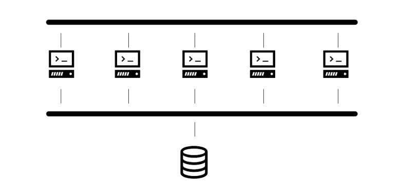
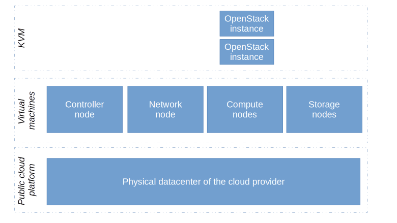
Therefore, I decided to use a slightly different approach on Packet which you might call the all-in-one approach – I simply moved my entire lab host into the cloud. Thus, I would get one sufficiently large bare metal server on Packet (with at least 32 GB of RAM, which is still quite affordable), install all the tools I would also need on my local lab host (Vagrant, VirtualBox, Ansible,..) and run the lab there as usual. Thus our OpenStack nodes are VirtualBox instances running on bare metal, and the instances that we bring up in Nova are using QEMU as nested virtualization on Intel CPUs is not supported by VirtualBox.

To automate this setup using Ansible, we can employ two stages. The first stage uses the Packet Ansible modules to create the lab host, set up the SSH configuration, install all the required software on the lab host, create a user and set up a basic firewall. We also need to install a few additional packages as the installation of VirtualBox will require some kernel modules to be built. In the second stage, we can then run the actual lab by fetching the latest version of the lab setup from the GitHub repository and invoking Vagrant and Ansible on the lab host.

If you want to try this, you will of course need a valid Packet.net account. Once you have that, head over to the Packet console and grab an API key. Put this API key into the environment variable PACKET_API_TOKEN. Next, create an SSH key pair called packet-default-key and place the private and public key in the .ssh subdirectory of your home directory. This SSH key will be added as authorized key to the lab host so that you can SSH into it. Finally, clone the GitHub repository and run the main playbook.

export PACKET_API_TOKEN=your packet.net token
ssh-keygen \
  -t rsa \
  -b 2048 \
  -f ~/.ssh/packet-default-key -P ""
git clone https://www.github.com/christianb93/openstack-labs
cd openstack-labs/Packet
ansible-playbook site.yaml

Be patient, this might take up to 30 minutes to complete, and in the last phase, when the actual lab is running on the remote host, you will not see any output from the main Ansible script. When the script completes, it will print a short message instructing you how the access the Horizon dashboard using an SSH tunnel to verify your setup.

By default, the script downloads and runs Lab6. You can change this by editing global_vars.yaml and setting the variable lab accordingly.

A distributed setup on GCP

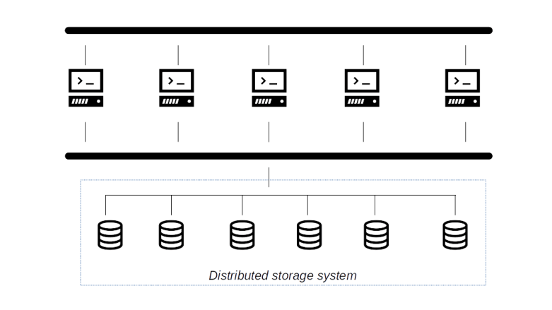
This all-in-one setup is useful, but actually not very flexible. It limits me to essentially one machine type (8 cores, 32 GB RAM), and when I ever needed more RAM I would have to choose a machine with 64 GB, thus doubling my bill. So I decided to try out a different setup – using virtual machines in a public cloud environment instead of having one large lab host, a setup which you might want to call a distributed setup.

Of course this comes at a price – we put a virtualized environment (compute and network) on top of another virtualized environment. To limit the impact of this, I was looking for a platform that supports nested virtualization with KVM, which would allow me to run KVM instead of QEMU as OpenStack hypervisor.

So I started to look at the various cloud providers that I typically use to understand my options. DigitalOcean seems to support nested virtualization with KVM, but is limited when it comes to network interfaces, at least I am not aware of a way how to add more than one additional network interface to a DigitalOcean droplet and to add more than one private network. AWS does not seem to support nested virtualization at all. Azure does, but only for HyperV. That left me with Google’s GCP platform.

GCP does, in fact, support nested virtualization with KVM. In addition, I can add an arbitrary number of public and private network interfaces to each instance, though this requires a minimum number of vCPUs, and GCP also offers custom instances with a flexible ratio of vCPUs and RAM. So I decided to give it a try.

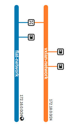
Next I started to design the layout of my networks. Obviously, a cloud platform implies some limitations for your networking setup. GCP, as most other public cloud platforms, does not provide layer 2 connectivity, but only layer 3 networking, so I would not be able to use flat or VLAN networks with Neutron, leaving overlay networks as the only choice. In addition, GCP does also not support IP multicast, which, however, is not a problem as the OVS based implementation of Neutron overlay networks only uses IP unicast messages. And GCP accepts VXLAN traffic (but does not support GRE encapsulation), so a Neutron overlay network using VXLAN should work.

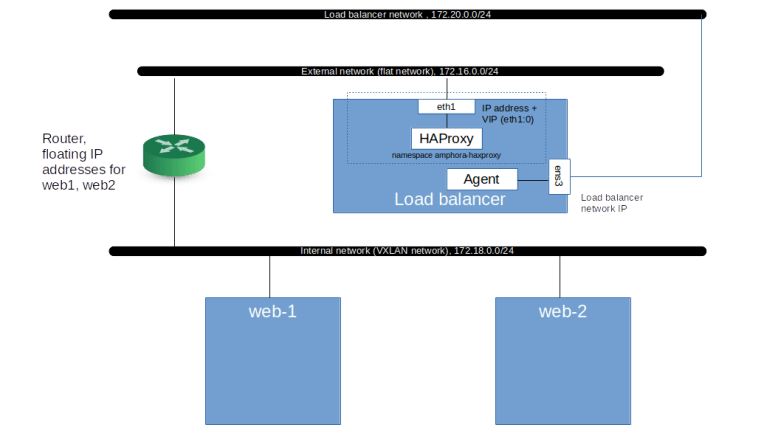
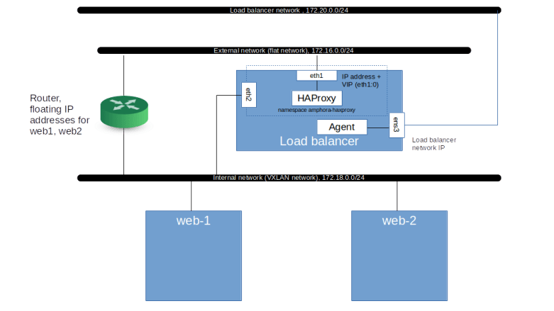
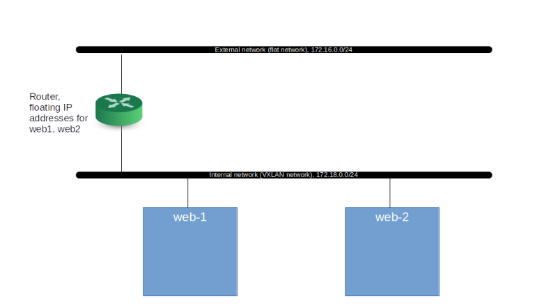
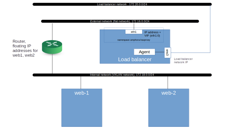
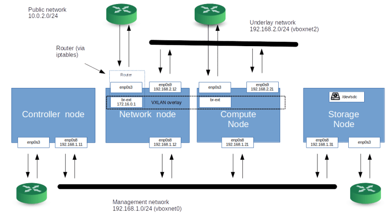
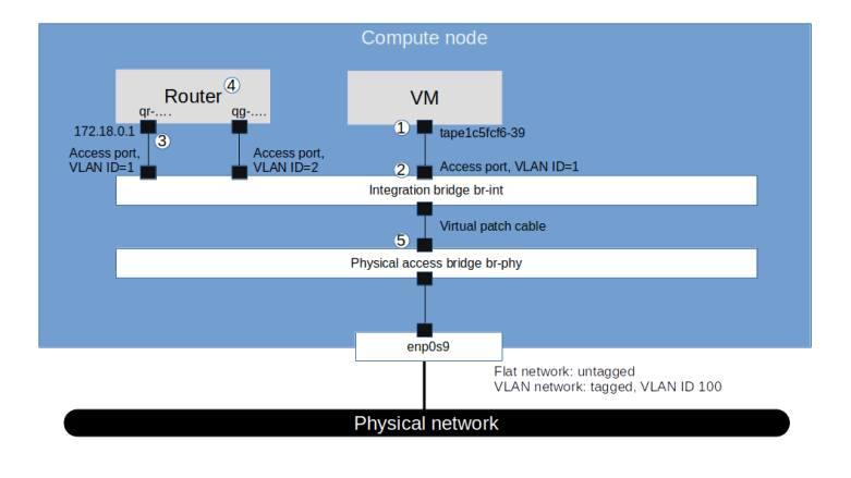
I was looking for a way to support at least three different GCP networks – a public network, which would provide access to the Internet from my nodes to download packages and to SSH into the machines, a management network to which all nodes would be attached and an underlay network that I would use to support Neutron overlay networks. As GCP only allows me to attach three network interfaces to a virtual machine with at least 4 vCPUs, I wanted to avoid a setup where each of the nodes would be attached to each network. Instead, I decided to put an APT cache on the controller node and to use the network node as SSH jump host for storage and compute nodes, so that only the network node requires four interfaces. To implement an external Neutron network, I use a OVS based VXLAN network across compute and network nodes which is presented as an external network to Neutron, as we have already done it in a previous post. Ignoring storage nodes, this leads to the following setup.

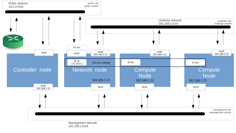
Of course, we need to be a bit careful with MTUs. As GCP does itself use an overlay network, the MTU of a standard GCP network device is 1460. When we add an additional layer of encapsulation to realize our Neutron overlay networks, we end up with an MTU of 1410 for the VNICs created inside the Nova KVM instances.

Automating the setup is rather straightforward. As demonstrated in a previous post, I use Terraform to bring up the base infrastructure and parse the Terraform output in my Ansible script to create a dynamic inventory. Then we set up the APT cache on the controller node (which, to avoid loops, implies that APT on the controller node must not use caching) and adapt the APT configuration on all other nodes to use it. We also use the network node as an SSH jump host (see this post for more on this) so that we can reach compute and storage nodes even though they do not have a public IP address.

Of course you will want to protect your machines using GCPs built-in firewalls (i.e. security groups). I have chosen to only allow incoming public traffic from the IP address of my own workstation (which also implies that you will not be able to use the GCP web based SSH console to reach your machines).

Finally, we need a way to access Horizon and the OpenStack API from our local workstation. For that purpose, I use an instance of NGINX running on the network host which proxies requests to the control node. When setting this up, there is a little twist – typically, a service like Keystone or Nova will return links in their responses, for instances to refer to entries in the service catalog or to the VNC proxy. These links will contain the IP address of our controller node, more specifically the management IP address of this node, which is not reachable from the public network. Therefore the NGINX forwarding rules need to rewrite these URLs to point to the network node – see the documentation of the Ansible role that I have written for this purpose for more details. The configuration uses SSL to secure the connection to NGINX so that the OpenStack credentials do not travel from your workstation to the network node unencrypted. Note, however, that in this setup, the traffic on the internal networks (the management network, the underlay network) is not encrypted.

To run this lab, there are of course some prerequisites. Obviously, you need a GCP account. It is also advisable to create a new project for this to be able to easily separate the automatically created resources from anything else you might have running on GCE. In the IAM console, make sure that your user has the “resourcemanager.organisationadministrator” role to be able to list and create new projects. Then navigate the to Manage Resources page, create a new project and create a service account for this new project. You will need to assign some roles to this service account so that it can create instances and networks – I use the compute instance admin role, the compute network admin role and the compute security admin role for that purpose.

To allow Terraform to create and destroy resources, we need the credentials of the service account. Use the GCP console to download a service account key in JSON format and store it on your local machine as ~/.keys/gcp_service_account.json. In addition, you will again have to create an SSH key pair and store it as ~/.ssh/gcp-default-key respectively ~/.ssh/gcp-default-key.pub, we will use this key to enable access to all GCP instances as user stack.

Once you are done with these preparations, you can now run the Terraform and Ansible scripts.

git clone https://www.github.com/christianb93/openstack-labs
cd openstack-labs/GCE
terraform init
terraform apply -auto-approve
ansible-playbook site.yaml
ansible-playbook demo.yaml

Once these scripts complete, you should be able to log into the Horizon console using the public IP of the network node, using the demo user credentials stored in ~/.os_credentials/credentials.yaml and see the instances created in demo.yaml up and running.

When you are done, you should clean up your resources again to avoid unnecessary charges. Thanks to Terraform, you can easily destroy all resources again using terraform destroy auto-approve.

OpenStack Octavia – creating listeners, pools and monitors

After provisioning our first load balancer in the previous post using Octavia, we will now add listeners and a pool of members to our load balancer to capture and route actual traffic through it.

Creating a listener

The first thing which we will add is called a listener in the load balancer terminology. Essentially, a listener is an endpoint on a load balancer reachable from the outside, i.e. a port exposed by the load balancer. To see this in action, I assume that you have followed the steps in my previous post, i.e. you have installed OpenStack and Octavia in our playground and have already created a load balancer. To add a listener to this configuration, let us SSH into the network node again and use the OpenStack CLI to set up our listener.

vagrant ssh network
source demo-openrc
openstack loadbalancer listener create \
  --name demo-listener \
  --protocol HTTP\
  --protocol-port 80 \
  --enable \
  demo-loadbalancer
openstack loadbalancer listener list
openstack loadbalancer listener show demo-listener

These commands will create a listener on port 80 of our load balancer and display the resulting setup. Let us now again log into the amphora to see what has changed.

amphora_ip=$(openstack loadbalancer amphora list \
  -c lb_network_ip -f value)
ssh -i amphora-key ubuntu@$amphora_ip
pids=$(sudo ip netns pids amphora-haproxy)
sudo ps wf -p $pids
sudo ip netns exec amphora-haproxy netstat -l -p -n -t

We now see a HAProxy inside the amphora-haproxy namespace which is listening on the VIP address on port 80. The HAProxy instance is using a configuration file in /var/lib/octavia/. If we display this configuration file, we see something like this.

# Configuration for loadbalancer bc0156a3-7d6f-4a08-9f01-f5c4a37cb6d2
global
    daemon
    user nobody
    log /dev/log local0
    log /dev/log local1 notice
    stats socket /var/lib/octavia/bc0156a3-7d6f-4a08-9f01-f5c4a37cb6d2.sock mode 0666 level user
    maxconn 1000000

defaults
    log global
    retries 3
    option redispatch
    option splice-request
    option splice-response
    option http-keep-alive

frontend 34ed8dd1-11db-47ee-a682-24a84d879d58
    option httplog
    maxconn 1000000
    bind 172.16.0.82:80
    mode http
    timeout client 50000

So we see that our listener shows up as a HAProxy frontend (identified by the UUID of the listener) which is bound to the load balancer VIP and listening on port 80. No forwarding rule has been created for this port yet, so traffic arriving there does not go anywhere at the moment (which makes sense, as we have not yet added any members). Octavia will, however, add our ports to the security group of the VIP to make sure that our traffic can reach the amphora. So at this point, our configuration looks as follows.

Adding members

Next we will add members, i.e. backends to which our load balancer will distribute traffic. Of course, the tiny CirrOS image that we use does not easily allow us to run a web server. We can, however, use netcat to create a “fake webserver” which will simply answer to each request with the same fixed string (I have first seen this nice little trick somewhere on StackExchange, but unfortunately I have not been able to dig out the post again, so I cannot provide a link and proper credits here). To make this work we first need to log out of the amphora again and, back on the network node, open port 80 on our internal network (to which our test instances are attached) so that traffic from the external network can reach our instances on port 80.

project_id=$(openstack project show \
  demo \
  -f value -c id)
security_group_id=$(openstack security group list \
  --project $project_id \
  -c ID -f value)
openstack security group rule create \
  --remote-ip 0.0.0.0/0 \
  --dst-port 80 \
  --protocol tcp \
  $security_group_id

Now let us create our “mini web server” on the first instance. The best approach is to use a terminal multiplexer like tmux to run this, as it will block the terminal we are using.

openstack server ssh \
  --identity demo-key \
  --login cirros --public web-1
# Inside the instance, enter:
while true; do
  echo -e "HTTP/1.1 200 OK\r\n\r\n$(hostname)" | sudo nc -l -p 80
done

Then, do the same on web-2 in a new session on the network node

source demo-openrc
openstack server ssh \
  --identity demo-key \
  --login cirros --public web-2
while true; do
  echo -e "HTTP/1.1 200 OK\r\n\r\n$(hostname)" | sudo nc -l -p 80
done

Now we have two “web server” running. Open another session on the network node and verify that you can reach both instances separately.

source demo-openrc
# Get floating IP addresses
web_1_fip=$(openstack server show \
  web-1 \
  -c addresses -f value | awk '{ print $2}')
web_2_fip=$(openstack server show \
  web-2 \
  -c addresses -f value | awk '{ print $2}')
curl $web_1_fip
curl $web_2_fip

So at this point, our web servers can be reached individually via the external network and the router (this is why we had to add the security group rule above, as the source IP of the requests will be an IP on the external network and thus would by default not be able to reach the instance on the internal network). Now let us add a pool, i.e. a set of backends (the members) between which the load balancer will distribute the traffic.

pool_id=$(openstack loadbalancer pool create \
  --protocol HTTP \
  --lb-algorithm ROUND_ROBIN \
  --enable \
  --listener demo-listener \
  -c id -f value)

When we now log into the loadbalancer again, we see that a backend configuration has been added to the HAProxy configuration, which will look similar to this sample.

backend af116765-3357-451c-8bf8-4aa2d3f77ca9:34ed8dd1-11db-47ee-a682-24a84d879d58
    mode http
    http-reuse safe
    balance roundrobin
    fullconn 1000000
    option allbackups
    timeout connect 5000
    timeout server 50000

However, there are still no real targets added to the backend, as the load balancer does not yet know about our web servers. As a last step, we now add these servers to the pool. At this point, it is important to understand which IP address we use. One option would be to use the floating IP addresses of the servers. Then, the target IP addresses would be on the same network as the VIP, leading to a setup which is known as “one armed load balancer”. Octavia can of course do this, but we will create a slightly more advanced setup in which the load balancer will also serve as a router, i.e. it will talk to the web servers on the internal network. On the network node, run

pool_id=$(openstack loadbalancer pool list \
  --loadbalancer demo-loadbalancer \
  -c id -f value)
for server in web-1 web-2; do
  ip=$(openstack server show $server \
       -c addresses -f value \
       | awk '{print $1'} \
       | sed 's/internal-network=//' \
       | sed 's/,//')
  openstack loadbalancer member create \
    --address $ip \
    --protocol-port 80 \
    --subnet-id internal-subnet \
    $pool_id
done
openstack loadbalancer member list $pool_id

Note that to make this setup work, we have to pass the additional parameter –subnet-id to the creation command for the members pointing to the internal network on which the specified IP addresses live, so that Octavia knows that this subnet needs to be attached to the amphora as well. In fact, we can see here that Octavia will add ports for all subnets which are specified via this parameter if the amphora is not yet connected to this subnet. Inside the amphora, the interface connected to this subnet will be added inside the amphora-haproxy namespace, resulting in the following setup.

If we now look at the HAProxy configuration file inside the amphora, we find that Octavia has added two server entries, corresponding to our two web servers. Thus we expect that traffic is load balanced to these two servers. Let us try this out by making requests to the VIP from the network node.

vip=$(openstack loadbalancer show \
  -c vip_address -f value \
   demo-loadbalancer)
for i in {1..10}; do 
  curl $vip;
  sleep 1
done

We see nicely that every second requests goes to the first server and every other request goes to the second server (we need a short delay between the requests, as the loop in our “fake” web servers needs time to start over).

Health monitors

This is nice, but there is an important ingredient which is still missing in our setup. A load balancer is supposed to monitor the health of the pool members and to remove members from the round-robin procedure if a member seems to be unhealthy. To allow Octavia to do this, we still need to add a health monitor, i.e. a health check rule, to our setup.

openstack loadbalancer healthmonitor create \
  --delay 10 \
  --timeout 10 \
  --max-retries 2 \
  --type HTTP \
  --http-method GET \
  --url-path "/" $pool_id

After running this, it is instructive to take a short look at the terminal in which our fake web servers are running. We will see additional requests, which are the health checks that are executed against our endpoints.

Now go back into the terminal on web-2 and kill the loop. Then let us display the status of the pool members.

openstack loadbalancer status show demo-loadbalancer

After a few seconds, the “operating_status” of the member changes to “ERROR”, and when we repeat the curl, we only get a response from the healthy server.

How does this work? In fact, Octavia uses the health check functionality that HAProxy offers. HAProxy will expose the results of this check via a Unix domain socket. The health daemon built into the amphora agent connects to this socket, collects the status information and adds it to the UDP heartbeat messages that it sends to the Octavia control plane via UDP port 5555. There, it is written into the various Octavia tables and finally collected again from the API server when we make our request via the OpenStack CLI.

This completes our last post on Octavia. Obviously, there is much more that could be said about load balancers, using a HA setup with VRRP for instance or adding L7 policies and rules. The Octavia documentation contains a number of cookbooks (like the layer 7 cookbook or the basic load balancing cookbook) that contain a lot of additional information on how to use these advanced features.

OpenStack Octavia – creating and monitoring a load balancer

In the last post, we have seen how Octavia works at an architectural level and have gone through the process of installing and configuring Octavia. Today, we will see Octavia in action – we will create our first load balancer and inspect the resulting configuration to better understand what Octavia is doing.

Creating a load balancer

This post assumes that you have followed the instructions in my previous post and run Lab14, so that you are now proud owner of a working OpenStack installation including Octavia. If you have not done this yet, here are the instructions to do so.

git clone https://www.github.com/christianb93/openstack-labs
cd openstack-labs/Lab14
wget https://s3.eu-central-1.amazonaws.com/cloud.leftasexercise.com/amphora-x64-haproxy.qcow2
vagrant up
ansible-playbook -i hosts.ini site.yaml

Now, let us bring up a test environment. As part of the Lab, I have provided a playbook which will create two test instances, called web-1 and web-2. To run this playbook, enter

ansible-playbook -i hosts.ini demo.yaml

In addition to the test instances, the playbook is creating a demo user and a role called load-balancer_admin. The default policy distributed with Octavia will grant all users to which this role is assigned the right to read and write load balancer configurations, so we assign this role to the demo user as well. The playbook will also set up an internal network to which the instances are attached plus a router, and will assign floating IP addresses to the instances, creating the following setup.

Once the playbook completes, we can log into the network node and inspect the running servers.

vagrant ssh network
source demo-openrc
openstack server list

Now its time to create our first load balancer. The load balancer will listen for incoming traffic on an address which is traditionally called virtual IP address (VIP). This terminology originates from a typical HA setup, in which you would have several load balancer instances in an active-passive configuration and use a protocol like VRRP to switch the IP address over to a new instance if the currently active instance fails. In our case, we do not do this, but still the term VIP is commonly used. When we create a load balancer, Octavia will assign a VIP for us and attach the load balancer to this network, but we need to pass the name of this network to Octavia as a parameter. With this, our command to start the load balancer and to monitor the Octavia log file to see how the provisioning process progresses is as follows.

openstack loadbalancer create \
  --name demo-loadbalancer\
  --vip-subnet external-subnet
sudo tail -f /var/log/octavia/octavia-worker.log

In the log file output, we can nicely see that Octavia is creating and signing a new certificate for use by the amphora. It then brings up the amphora and tries to establish a connection to its port 9443 (on which the agent will be listening) until the connection succeeds. If this happens, the instance is supposed to be ready. So let us wait until we see a line like “Mark ACTIVE in DB…” in the log file, hit ctrl-c and then display the load balancer.

openstack loadbalancer list
openstack loadbalancer amphora list

You should see that your new load balancer is in status ACTIVE and that an amphora has been created. Let us get the IP address of this amphora and SSH into it.

amphora_ip=$(openstack loadbalancer amphora list \
  -c lb_network_ip -f value)
ssh -i amphora-key ubuntu@$amphora_ip

Nice. You should now be inside the amphora instance, which is running a stripped down version of Ubuntu 16.04. Now let us see what is running inside the amphora.

ifconfig -a
sudo ps axwf
sudo netstat -a -n -p -t -u

We find that in addition to the usual basic processes that you would expect in every Ubuntu Linux, there is an instance of the Gunicorn WSGI server, which runs the amphora agent, listening on port 9443. We also see that the amphora agent holds a UDP socket, this is the socket that the agent uses to send health messages to the control plane. We also see that our amphora has received an IP address on the load balancer management network. It is also instructive to display the configuration file that Octavia has generated for the agent – here we find, for instance, the address of the health manager to which the agent should send heartbeats.

This is nice, but where is the actual proxy? Based on our discussion of the architecture, we would have expected to see a HAProxy somewhere – where is it? The answer is that Octavia puts this HAProxy into a separate namespace, to avoid potential IP address range conflicts between the subnets on which HAProxy needs to listen (i.e. the subnet on which the VIP lives, which is specified by the user) and the subnet to which the agent needs to be attached (the load balancer management network, specified by the administrator). So let us look for this namespace.

ip netns list

In fact, there is a namespace called amphora-haproxy. We can use the ip netns exec command and nsenter to take a look at the configuration inside this namespace.

sudo ip netns exec amphora-haproxy ifconfig -a

We see that there is a virtual device eth1 inside the namespace, with an IP address on the external network. In addition, we see an alias on this device, i.e. essentially a second IP address. This the VIP, which could be detached from this instance and attached to another instance in an HA setup (the first IP is often called the VRRP address, again a term originating from its meaning in a HA setup as being the IP address of the interface across which the VRRP protocol is run).

At this point, no proxy is running yet (we will see later that the proxy is started only when we create listeners), so the configuration that we find is as displayed below.

Monitoring load balancers

We have mentioned several times that the agent is send hearbeats to the health manager, so let us take a few minutes to dig into this. During the installation, we have created a virtual device called lb_port on our network node, which is attached to the integration bridge to establish connectivity to the load balancer management network. So let us log out of the amphora to get back to the network node and dump the UDP traffic crossing this interface.

sudo tcpdump -n -p udp -i lb_port

If we look at the output for a few seconds, then we find that every 10 seconds, a UDP packet arrives, coming from the UDP port of the amphora agent that we have seen earlier and the IP address of the amphora on the load balancer management network, and targeted towards port 5555. If you add -A to the tcpdump command, you find that the output is unreadable – this is because the heartbeat message is encrypted using the heartbeat key that we have defined in the Octavia configuration file. The format of the status message that is actually sent can be found here in the Octavia source code. We find that the agent will transmit the following information as part of the status messages:

The ID of the amphora
A list of listeners configured for this load balancer, with status information and statistics for each of them
Similarly, a list of pools with information on the members that the pool contains

We can display the current status information using the OpenStack CLI as follows.

openstack loadbalancer status show demo-loadbalancer
openstack loadbalancer stats show demo-loadbalancer

At the moment, this is not yet too exciting, as we did not yet set up any listeners, pools and members for our load balancer, i.e. our load balancer is not yet accepting and forwarding any traffic at all. In the next post, we will look in more detail into how this is done.

OpenStack Octavia – architecture and installation

Once you have a cloud platform with virtual machines, network and storage, you will sooner or later want to expose services running on your platform to the outside world. The natural way to do this is to use a load balancer, and in a cloud, you of course want to utilize a virtual load balancer. For OpenStack, the Octavia project provides this as a service, and in todays post, we will take a look at Octavias architecture and learn how to install it.

Octavia components

When designing a virtual load balancer, one of the key decisions you have to take is where to place the actual load balancer functionality. One obvious option would be to spawn software load balancers like HAProxy or NGINX on one of the controller nodes or the network node and route all traffic via those nodes. This approach, however, has the clear disadvantage that it introduces a single point of failure (unless, of course, you run your controller nodes in a HA setup) and, even worse, it puts a load of load on the network interfaces of these few nodes, which implies that this solution does not scale well when the number of virtual load balancers or endpoints increases.

Octavia chooses a different approach. The actual load balancers are realized by virtual machines, which are ordinary OpenStack instances running on the compute nodes, but use a dedicated image containing a HAProxy software load balancer and an agent used to control the configuration of the HAProxy instance. These instances – called the amphorae – are therefore scheduled by the Nova scheduler as any other Nova instances and thus scale well as they can leverage all available compute nodes. To control the amphorae, Octavia uses a control plane which consists of the Octavia worker running the logic to create, update and remove load balancers, the health manager which monitors the amphorae and the house keeping service which performs clean up activities and can manage a pool of spare amphorae to optimize the time it takes to spin up a new load balancer. In addition, as any other OpenStack project, Octavia exposes its functionality via an API server.

The API server and the control plane components communicate with each other using RPC calls, i.e. RabbitMQ, as we have already seen it for the other OpenStack services. However, the control plane components also have to communicate with the amphorae. This communication is bi-directional.

The agent running on each amphora exposes a REST API that the control plane needs to be able to reach
Conversely, the health manager listens for health status messages issued by the amphorae and therefore the control plane needs to be reachable from the amphorae as well

To enable this two-way communication, Octavia assumes that there is a virtual (i.e. Neutron) network called the load balancer management network which is specified by the administrator during the installation. Octavia will then attach all amphorae to this network. Further, Octavia assumes that via this network, the control plane components can reach the REST API exposed by the agent running on each amphora and conversely that the agent can reach the control plane via this network. There are several ways to achieve this, we get back to this point when discussing the installation further below. Thus the overall architecture of an Octavia installation including running load balancers is as in the diagram below.

Octavia installation

Large parts of the Octavia installation procedure (which, for Ubuntu, is described here in the official documentation) is along the lines of the installation procedures for other OpenStack components that we have already seen – create users, database tables, API endpoints, configure and start services and so forth. However, there are a few points during the installation where I found that the official documentation is misleading (at the least) or where I had problems figuring out what was going on and had to spend some time reading source code to clarify a few things. Here are the main pitfalls.

Creating and connecting the load balancer management network

The first challenge is the setup of the load balancer network mentioned before. Recall that this needs to be a virtual network to which our amphorae will attach which allows access to the amphorae from the control plane and allows traffic from the amphorae to reach the health manager. To build this network, there are several options.

First, we could of course create a dedicated provider network for this purpose. Thus, we would reserve a physical interface or a VLAN tag on each node for that network and would set up a corresponding provider network in Neutron which we use as load balancer management network. Obviously, this only works if your physical network infrastructure allows for it.

If this is not the case, another option would be to use a “fake” physical network as we have done it in one of our previous labs. We could, for instance, set up an OVS bridge managed outside of Neutron on each node, connect these bridges using an overlay network and present this network to Neutron as a physical network on which we base a provider network. This should work in most environments, but creates an additional overhead due to the additionally needed bridges on each node.

Finally – and this is the approach that also the official installation instructions take – we could simply use a VXLAN network as load balancer management network and connect to it from the network node by adding an additional network device to the Neutron integration bridge. Unfortunately, the instructions provided as part of the official documentation only work if Linux bridges are used, so we need to take a more detailed look at this option in our case (using OVS bridges).

Recall that if we set up a Neutron VXLAN network, this network will manifest itself as a local VLAN tag on the integration bridge of each node on which a port is connected to this network. Specifically, this is true for the network node, on which the DHCP agent for our VXLAN network will be running. Thus, when we create the network, Neutron will spin up a DHCP agent on the network node and will assign a local VLAN tag used for traffic belonging to this network on the integration bridge br-int.

To connect to this network from the network node, we can now simply bring up an additional internal port attached to the integration bridge (which will be visible as a virtual network device) and configured access port, using this VLAN tag. We then assign an IP address to this device, and using this IP address as a gateway, we can now connect to every other port on the Neutron VXLAN network from the network node. As the Octavia control plane components communicate with the Octavia API server via RPC, we can place them on the network node so that they can use this interface to communicate with the amphorae.

With this approach, the steps to set up the network are as follows (see also the corresponding Ansible script for details).

Create a virtual network as an ordinary Neutron VXLAN network and add a subnet
Create security groups to allow traffic to the TCP port on which the amphora agent exposes its REST API (port 9443 by default) and to allow access to the health manager (UDP, port 5555). It is also helpful to allow SSH and ICMP traffic to be able to analyze issues by pinging and accessing the amphorae
Now we create a port on the load balancer network. This will reserve an IP address that we can use for our port to avoid IP address conflicts with Neutron
Then we wait until the namespace for the DHCP agent has been created, get the ID of the corresponding Neutron port and read the VLAN tag for this port from the OVS DB (I have created a Jinja2 template to build a script doing all this)
Now create an OVS access port using this VLAN ID, assign an IP address to the corresponding virtual network device and bring up the device

There is a little gotcha with this configuration when the OVS agent is restarted, as in this case, the local VLAN ID can change. Therefore we also need to create a script to refresh the configuration and run it via a systemd unit file whenever the OVS agent is restarted.

Image creation

The next challenge I was facing during the installation was the creation of the image. Sure, Octavia comes with instructions and a script to do this, but I found some of the parameters a bit difficult to understand and had to take a look at the source code of the scripts to figure out what they mean. Eventually, I wrote a Dockerfile to run the build in a container and corresponding instructions. When building and running a container with this Dockerfile, the necessary code will be downloaded from the Octavia GitHub repository, some required tools are installed in the container and the image build script is started. To have access to the generated image and to be able to cache data across builds, the Dockerfile assumes that your local working directory is mapped into the container as described in the instructions.

Once the image has been built, it needs to be uploaded into Glance and tagged with a tag that will also be added to the Octavia configuration. This tag is later used by Octavia when an amphora is created to locate the correct image. In addition, we will have to set up a flavor to use for the amphorae. Note that we need at least 1 GB of RAM and 2 GB of disk space to be able to run the amphora image, so make sure to size the flavor accordingly.

Certificates, keys and configuration

We have seen above that the control plane components of Octavia use a REST API exposed by the agent running on each amphora to make changes to the configuration of the HAProxy instances. Obviously, this connection needs to be secured. For that purpose, Octavia uses TLS certificates.

First, there is a client certificate. This certificate will be used by the control plane to authenticate itself when connecting to the agent. The client certificate and the corresponding key need to be created during installation. As the CA certificate used to sign the client certificate needs to be present on every amphora (so that the agent can use it to verify incoming requests), this certificate needs to be known to Octavia as well, and Octavia will distribute it to each newly created amphora.

Second, each agent of course needs a server certificate. These certificates are unique to each agent and are created dynamically at run time by a certificate generator built into the Octavia control plane. During the installation, we only have to provide a CA certificate and a corresponding private key which Octavia will then use to issue the server certificates. The following diagram summarizes the involved certificates and key.

In addition, Octavia can place an SSH key on each amphora to allow us to SSH into an amphora in case there are any issues with it. And finally, a short string is used as a secret to encrypt the health status messages. Thus, during the installation, we have to create

A root CA certificate that will be placed on each amphora
A client certificate signed by this root CA and a corresponding client key
An additional root CA certificate that Octavia will use to create the server certificates and a corresponding key
An SSH key pair
A secret for the encryption of the health messages

More details on this, how these certificates are referenced in the configuration and a list of other relevant configuration options can be found in the documentation of the Ansible role that I use for the installation.

Versioning issues

During the installation, I came across an interesting versioning issue. The API used to communicate between the control plane and the agent is versioned. To allow different versions to interact, the client code used by the control plane has a version detection mechanism built into it, i.e. it will first ask the REST API for a list of available versions and then pick one based on its own capabilities. This code obviously was added with the Stein release.

When I first installed Octavia, I used the Ubuntu packages for the Stein release which are part of the Ubuntu Cloud archive. However, I experienced errors when the control plane was trying to connect to the agents. During debugging, I found that the versioning code is present in the Stein branch on GitHub but not included in the version of the code distributed with the Ubuntu packages. This, of course, makes it impossible to establish a connection.

I do not know whether this is an archiving error or whether the versioning code was added to the Stein maintenance branch after the official release had gone out. To fix this, I now pull the source code once more from GitHub when installing the Octavia control plane to make sure that I run the latest version from the Stein GitHub branch.

Lab 14: adding Octavia to our OpenStack playground

After all this theory, let us now run Lab14, in which we add Octavia to our OpenStack playground. Obviously, we need the amphora image to do this. You can either follow the instructions above to build your own version of the image, or you can use a version which I have built and uploaded into an S3 bucket. The instructions below use this version.

So to run the lab, enter the following commands (assuming, as always in this series, that you have gone through the basic setup described here).

git clone https://www.github.com/christianb93/openstack-labs
cd openstack-labs/Lab14
wget https://s3.eu-central-1.amazonaws.com/cloud.leftasexercise.com/amphora-x64-haproxy.qcow2
vagrant up
ansible-playbook -i hosts.ini site.yaml

In the next post, we will test this setup by bringing up our first load balancer and go through the configuration and provisioning process step by step.

OpenStack Cinder – creating and using volumes

In the previous post, we have installed Cinder and described its high level architecture. Today, we will look at a few uses cases (creating and attaching volumes) in detail, go through the code and see how Cinder interacts with external technologies like iSCSI and LVM.

Creating a volume

Let us first try to understand what happens when a volume is created, for instance because a user submit the corresponding API request via the OpenStack CLI, using v3 of the API.

In the architecture overview, we have mentioned that the Cinder API server is run by Apache. To understand how this request is processed, it therefore makes sense to start at the Apache2 configuration in /etc/apache2/conf-available/cinder-wsgi.conf. Here, we find a reference to the script cinder-wsgi which in turn shows up in the setup.cfg file distributed with Cinder. Following the link in this file, we find that the WSGI server is initialized by initialize_application which in turn uses the Oslo service library to create an application from a PasteDeploy configuration.

Browsing the PasteDeploy config that is distributed with Cinder, we find that, as we have seen it before, it defines several authorization strategies. We use the Keystone strategy, and in this pipeline, the last element points to the factory method cinder.api.v3.router.APIRouter.factory, implemented here. This class implements a routing mechanism, which translates our PUT request into a call to VolumeController.create.

So far, this flow looks familiar and we have seen this before – there is a WSGI application acting as an API endpoint, which routes requests to various controller. Now the Cinder specific processing starts, and the Controller, after performing some transformations and validations, invokes cinder.volumes.API().create()

This method now uses a device which we can find at several points in OpenStack when it comes to managing processes consisting of several steps – the OpenStack Taskflow library. This library provides flows that can be built from tasks, can be run using a flow engine and can be stopped and reverted in a controlled manner. In Cinder, various processes are modeled as flows. In our case, the flow is built by this method and consists of several tasks, which will deduct the volume size from the quota, create a database object for the volume and commit the changed quota. If everything succeeds, we now delegate to the scheduler for further processing by triggering a RPC call via RabbitMQ.

The entry point into the scheduler, which is running as an independent process, is the method create_volume of the corresponding manager object cinder.scheduler.SchedulerManager. Here, we create another flow and run it. This flow does again do some validation and then calls a scheduler driver, which, as so often in OpenStack, is a pluggable module that carries out the actual scheduling. In our case, this is the filter scheduler. After the actual scheduling is complete, the driver now sends an RPC call to the selected node which is received by the volume manager, more precisely by its method create_volume.

This again creates a flow, which will include a task that does the actual volume creation (CreateVolumeFromSpecTask). Here, the actual work is delegated to a volume driver. In our setup, our driver is the LVM driver (cinder.volume.drivers.LVMVolumeDriver). We first look at its _init_ method. Here we determine the target_helper from the configuration and create the corresponding target driver. During initialization, the manager will also call the method check_for_setup_error which, among other things, creates an object which represents the volume group that Cinder manages and which is an instance of cinder.brick.local_dev.LVM. When the method create_volume of the volume driver is called, it will essentially delegate the call to this class. In its create_volume method, we now finally see that the LVM command lvcreate is called which creates the actual logical volume.

Let us try to find the traces of all this in our setup. For that purpose, re-start the setup from the previous setup, and, if you have not yet done so, create a volume of size 1 (GB).

git clone https://github.com/christianb93/openstack-labs
cd openstack-labs/Lab13
vagrant up
ansible-playbook -i hosts.ini site.yaml
ansible-playbook -i hosts.ini demo.yaml
vagrant ssh network
source demo-openrc
openstack volume create \
  --size 1 \
  demo-volume

Now log out of the network node, log into the storage node and run sudo lvs. You should see two volumes, both on top of the volume group cinder-volumes, as in the sample output below.

  LV                                          VG             Attr       LSize Pool                Origin Data%  Meta%  Move Log Cpy%Sync Convert
  cinder-volumes-pool                         cinder-volumes twi-aotz-- 4.75g                            0.00   10.64                           
  volume-5eae9e4b-6a28-41a2-a983-e435ec23ce46 cinder-volumes Vwi-a-tz-- 1.00g cinder-volumes-pool        0.00

We see that there is a new logical volume, whose name is the prefix volume-, followed by the UUID of the volume that we have just created. This is a so-called thin volume, meaning that LVM does not allocate extends when the logical volume is created, but maintains a pool of available extends and allocates extends from this pool only when data is actually written. This is a sort of over-commitment of storage, as it allows us to create volumes which have a size much larger than the actually physically available size.

Attaching a volume

At this point, we have created a virtual storage volume which is living on the storage node. In order to be usable for an instance, we now have to attach the volume to an instance. Before trying this out, let us again see how this request will flow through the source code.

Typically, attaching a volume is done by a call to the Nova API. Nova will then in turn call the Cinder API where the calls will be processed by the Cinder attachment controller. Actually, during the process of attaching a volume to an instance, Nova will invoke the Cinder API three times (not counting read-only requests). First, it will use a POST request to ask the controller to create the attachment, then it will use a PUT request to update the attachment by providing so-called connector information and finally, it will use another POST request to call the complete method to signal that the process of attaching the volume is complete.

Let us start to understand the first request. Here, Nova only provides the UUID of the volume and the UUID of the instance to be connected. This request will be served by the create method of the attachment controller. After some preparations, the controller will then invoke the method attachment_create of the volume manager API. At this point, no connector information is available yet, so all this method does is to create a reservation by storing the attachment in the database.

Now the second call from Nova comes in. At this point, Nova will have collected the connector information, which is the IP address of the compute node, the iSCSI initiator name, the mount point and some additional information. Just in case you want to link this back into the Nova code: the connector data is assembled here (where we can also see that the IP address used is taken from the configuration item my_block_storage_ip in the Nova configuration), and the update call to the Cinder API which we are currently discussing is made here.

A typical connector information could look as follows.

{'connector': 
  {'platform': 'x86_64', 
   'os_type': 'linux', 
   'ip': '192.168.1.21', 
   'host': 'compute1', 
   'multipath': False, 
   'initiator': 'iqn.1993-08.org.debian:01:a41db8382266', 
   'do_local_attach': False, 
   'system uuid': '54F9944F-66C9-411E-9989-84AB5CEE6B18', 
   'mountpoint': '/dev/vdc'}
}

The update call will again reach the volume manager API which will look up the volume and forward the request via RPC to the volume manager on the storage node where the storage is located. The result – the connection information – is then returned to the callee, i.e. in our case the Nova driver, which then connects to the device using a volume driver and eventually submits the third call to Cinder to signal completion.

But let us continue to investigate the call chain for the update call first. The volume manager on the storage node now performs several steps. First, it calls the responsible Cinder volume driver (which, in our case, is the LVM driver) to create the export, i.e. to activate the logical volume and to use a target driver to initiate the actual export. In our case, the target driver is the iSCSI driver, and export here simply means that an iSCSI target is created on the storage driver (and a CHAP secret is returned).

Back in the volume manager, the manager next calls the method initialize_connection of the driver which is simply passed through to the target driver and assembles the connection information, i.e. the target and portal information. Finally, the manager makes a call to the method attach_volume of the volume driver, but this method is empty for the LVM driver. At this point, the database record is updated and the connection info is returned.

Nova is now able to finalize the attachment by using the Open-iSCSI helper to establish the connection to the target using iscsiadmin from the Open-iSCSI package. When all this succeeds, Nova will eventually call Cinder a third time, this time invoking the complete method of the attachment controller. This method will update the attachment and the volume in the database, and the entire process is complete.

Let us now try to identify some of the objects created during this process in our lab setup. For that purpose, first log into the networking node and attach the volume that we have just created to our instance.

source demo-openrc
openstack server \
  add volume \
  demo-instance-3 \
  demo-volume

Now log out off the network node and log into the compute node. Here, we first use iscsiadm to display all open iSCSI sessions.

sudo iscsiadm -m session -P 3

Here you can see that we have an open session connected to the iSCSI target that Cinder has created for this volume, and you can see that this volume is mapped to a block device like /dev/sdc on the compute node. Note that there is actually one target for each volume, so that a dedicated CHAP secret can be used for every logical volume.

Now let us try to locate this block device in the configuration of our KVM/QEMU guest. For this purpose, we first use the OpenStack API to determine the UUID of the instance and then the virsh manager to display this instance.

source demo-openrc
uuid=$(openstack server show \
  demo-instance-3 \
  -c id -f value)
sudo virsh domblklist $uuid

We now see that the instance has two devices attached to it. The first device is mapped to /dev/vda inside the instance and is the root device. This device is a flat file that Nova has created and placed on the compute host, i.e. it is an ephemeral device which gets lost if the instance is destroyed, the host goes down or the instance is migrated to a different machine. The second device is our device /dev/sdc which is pointing via iSCSI to the virtual device on the storage node.

There are many other functions of Cinder that we have not yet touched upon. You can, for instance, create volumes from existing images, in which case Glance comes into play, or Cinder can use the snapshot functionality of LVM to create and manage snapshots. It is also possible to configure Cinder such that is uses mirrored LVM devices (with a local mirror, though), and of course there are many other volume drivers apart from LVM. Going through all this would be a separate series, but I hope that I could at least provide some entry points into code and documentation so that you can explore all this if you want.

OpenStack Cinder – architecture and installation

Having looked at the foundations of the storage technology that Cinder uses in the previous posts, we are now ready to explore the basic architecture of Cinder and install Cinder in our playground.

Cinder architecture

Essentially, Cinder consists of three main components which are running as independent processes and typically on different nodes.

First, there is the Cinder API server cinder-api. This is a WSGI-server running inside of Apache2. As the name suggests, cinder-api is responsible for accepting and processing REST API requests from users and other components of OpenStack and typically runs on a controller node.

Then, there is cinder-volume, the Cinder volume manager. This component is running on each node to which storage is attached (“storage node”) and is resonsible for managing this storage, i.e. preparing, maintaining and deleting virtual volumes and exporting these volumes so that they can be used by a compute node. And finally, Cinder comes with its own scheduler, which directs requests to create a virtual volume to an appropriate storage node.

Of course, Cinder also has its own database and communicates with other components of OpenStack, for example with Keystone to authenticate requests and with Glance to be able to create volumes from images.

Cinder van use a variety of different storage backends, ranging from LVM managing local storage directly attached to a storage node over other standards like NFS and open source solutions like Ceph to vendor-specific drivers like Dell, Huawei, NetApp or Oracle – see the official support matrix for a full list. This is achieved by moving low-level access to the actual volumes into a volume driver. Similarly, Cinder uses various technologies to connect the virtual volumes to the compute node on which an instance that wants to use it is running, using a so-called target driver.

To better understand how Cinder operates, let us take a look at one specific use case – creating a volume and attaching to an instance. We will go in more detail on this and similar use cases in the next post, but what essentially happens is the following:

A user (for instance an administrator) sends a request to the Cinder API server to create a logical volume
The API server asks the scheduler to determine a storage node with sufficient capacity
The request is forwarded to the volume manager on the target node
The volume manager uses a volume driver to create a logical volume. With the default settings, this will be LVM, for which a volume group and underlying physical volumes have been created during installation. LVM will thzen create a new logical volume
Next, the administrator attaches the volume to an instance using another API request
Now, the target driver is invoked which sets up an iSCSI target on the storage node and a LUN pointing to the logical volume
The storage node informs the compute node about the parameters (portal IP and port, target name) that are needed to access this target
The Nova compute agent on the compute node invokes an iSCSI initiator which maps the iSCSI target into the local file system
Finally, the Nova compute agent asks the virtual machine driver (libvirt in our case) to attach this locally mapped device to the instance

Installation steps

After this short summary of the high-level architecture of Cinder, let us move and try to understand how the installation process looks like. Again, the installation follows the standard pattern that we have now seen so many times.

Create a database for Cinder and prepare a database user
Add user, services and endpoints in Keystone
Install the Cinder packages on the controller and the storage nodes
Modify the configuration files as needed

In addition to these standard steps, there are a few points specific for Cinder. First, as sketched above, Cinder uses LVM to manage virtual volumes on the storage nodes. We therefore need to perform a basic setup of LVM on each storage node, i.e. we need to create physical volumes and a volume group. Second, every compute node will need to act as iSCSI initiator and therefore needs a valid iSCSI initiator name. The Ubuntu distribution that we use already contains the Open-iSCSI package, which maintains an initiator name in the file /etc/iscsi/initiatorname.iscsi. However, as this name is supposed to be unique, it is not set in the Ubuntu Vagrant image and we need to do this once during the installation by running the script /lib/open-iscsi/startup-checks.sh as root.

There is an additional point that we need to observe which is also not mentioned in the official installation guide for the Stein release. When installing Cinder, you have to define which network interface Cinder will use for the iSCSI traffic. In production, you would probably want to use a separate storage network, but for our setup, we use the management network. According to the installation guide, it should be sufficient to set the configuration item my_ip, but in reality, this did not work for me and I had to set the item target_ip_address on the storage nodes.

Lab13: running and testing the Cinder installation

Time to try this out and set up a lab for that. The first thing we need to do is to modify our Vagrantfile to add a storage node. In order to reduce memory consumption a bit, we instead move from having two computes to one compute node only, so that our new setup looks as follows.

As mentioned above, we will not use a dedicated storage network, but send the iSCSI traffic over the management network so that our network setup remains essentially unchanged. To bring up this scenario and to run the Cinder installation plus a demo setup do the following.

git clone https://github.com/christianb93/openstack-labs
cd openstack-labs/Lab13
vagrant up
ansible-playbook -i hosts.ini site.yaml
ansible-playbook -i hosts.ini demo.yaml

When all this completes, we can run some tests. First, verify that all storage nodes are up and running. For that purpose, log into the controller node and use the OpenStack CLI to retrieve a list of all recognized storage nodes.

vagrant ssh controller
source admin-openrc
openstack volume service list

The output that you get should look similar to the sample output below.

+------------------+-------------+------+---------+-------+----------------------------+
| Binary           | Host        | Zone | Status  | State | Updated At                 |
+------------------+-------------+------+---------+-------+----------------------------+
| cinder-scheduler | controller  | nova | enabled | up    | 2020-01-01T14:03:14.000000 |
| cinder-volume    | storage@lvm | nova | enabled | up    | 2020-01-01T14:03:14.000000 |
+------------------+-------------+------+---------+-------+----------------------------+

We see that there are two services that have been detected. First, there is the Cinder scheduler running on the controller node, and then, there is the Cinder volume manager on the storage node. Both are “up”, which is promising.

Next, let us try to create a volume and attach it to one of our test instances, say demo-instance-3. For this to work, you need to be on the network node (as we will have to establish connectivity to the instance).

vagrant ssh network
source demo-openrc
openstack volume create \
  --size=1 \
  demo-volume
openstack server add volume \
  demo-instance-3 \
  demo-volume
openstack server show demo-instance-3
openstack server ssh \
  --identity demo-key \
  --login cirros \
  --private demo-instance-3

You should now be inside the instance. When you run lsblk, you should find a new block device /dev/vdb being added. So our installation seems to work!

Having a working testbed, we are now ready to dive a little deeper into the inner workings of Cinder. In the next post, we will try to understand some of the common use cases in a bit more detail.

OpenStack Cinder foundations – storage networks, iSCSI, LUNs and all that

To understand Cinder, the block device component of OpenStack, you will need to be familiar with some terms that originate from the world of data center networks like SCSI, SAN, LUN and so forth. In this post, we will take a short look at these topics to be prepared for our upcoming installation and configuration of Cinder.

Storage networks

In the early days of computing, when persistent mass storage was introduced, storage devices where typically directly attached to a server, similar to the hard disk in your PC or laptop computer which is sitting in same enclosure as your motherboard and directly connected to it. In order to communicate with such a storage device, there would usually be some sort of controller on the motherboard which would use some low-level protocol to talk to a controller on the storage device.

A protocol to achieve this which is (still) very popular in the world of Intel PCs is the SATA protocol, but this is by far not the only one. In most enterprise storage solutions, another protocol called SCSI (small computer system interface) is still dominating, which was originally also used in the consumer market by companies like Apple. Let us quickly summarize some terms that are relevant when dealing with SCSI based devices.

First, every device on a SCSI bus has a SCSI ID. As a typical SCSI storage device may expose more than one disk, these disks are represented by logical unit numbers (LUNs). Generally speaking, every object that can receive a SCSI command is a logical unit (there are also logical units that do not represent actuals disks, but controllers). Each SCSI device can encompass more than one LUN. A SCSI device could, for instance, be a RAID array that exposes two logical disks, and each of these disks would then be addressable as a separate LUN.

When devices communicate over the SCSI bus, one of them acts as initiator and one of them acts as target. If, for instance, a host controller wants to read data from a SCSI hard disk, the host controller is the initiator, and the controller of the hard disk is the target. The initiator can send commands like “read a block” to the target, and the target will reply with data and / or a status code.

Now imagine a data center in which there is a large number of servers, each of which being equipped with a direct attached storage device.

The servers might be connected by a network, but each disk (or other storage device like tape or a removable media drive) is only connected to one server. This setup is simple, but has a couple of drawbacks. First, if there is some space available on a disk, it cannot easily be made available for other servers, so that the overall utilization is low. Second, topics like availability, redundancy, backups, proper cooling and so forth have to be done individually for each server. And, last but not least, physical maintenance can be difficult if the servers are distributed over several locations.

For those reasons, an alternative architecture has evolved over time, in which storage capacity is centralized. Instead of having one disk attached to each server, most of the storage capacity is moved into a central storage appliance. This appliance is then connected to each server via a (typically dedicated) network, hence the term SAN – storage attached network that describes this sort of architecture (often, each server would still have a small disk as a primary partition for the operating system and booting, but not even this is actually required).

Of course, the storage in such a scenario is typically not just an ordinary disk, but an entire array of disks, combined into a RAID array for better performance and redundancy, and often equipped with some additional capabilities like de-duplication, instant copy, a management interface and so forth.

Very often, storage networks are not based on Ethernet and IP, but on the FibreChannel network protocol stack. However, there is also a protocol called iSCSI which can be used to run SCSI on top of TCP/IP, so that a SAN can be leveraging existing IP-based networks and technologies – more on this in the next section.

Finally, there is a third possible architecture (which we do not discuss in detail in this post), which is becoming increasingly popular in the context of cloud and container platforms – distributed storage systems. With this approach, storage is still separated from the compute capacity and connected using a network, but instead of having a small number of large storage appliances that pool the available storage capacity, these solutions take a comparatively large number of smaller nodes, often commodity hardware, which distribute and replicate data to form a large, highly available virtual storage system. Examples for this type of solutions are the HDFS file system used by Hadoop, Ceph or GlusterFS.

The iSCSI protocol

Let us now take a closer look at the iSCSI protocol. This protocol, standardized in RFC 7143 (which is replacing earlier RFCs), is a transport protocol for SCSI which can be used to build storage networks utilizing SCSI capable devices based on an underlying IP network.

In an iSCSI setup, an iSCSI initiator talks to an iSCSI target using one or more TCP/IP connections. The combination of all active sessions between an initiator and a target is called a session, and is roughly equivalent to what is known as I_T nexus (initiator – target nexus) in the SCSI protocol. Each session is identified by a session ID, and each connection within a session has a connection ID. Logically, a session describes an ongoing communication between an initiator and a target, but the traffic can be spread across several TCP/IP connections to support redundancy and failover.

Both, the initiator and the target, are identified by a unique name. The RFC defines several ways to build iSCSI names. One approach is to use a combination of

The qualifier iqn to mark the name as an iSCSI qualified name
a (reversed) domain name which is supposed to be owned by whoever assigns the name so that the resulting name will be unique
a date (yyyy-mm) between the leading iqn and the domain name which is a date at which the domain ownership was valid (to be able to deal with changing domain name ownerships)
A colon followed by a postfix to make the name unique within the domain

As I own the domain leftasexercise.com since 2018, an example for a iSCSI name that I could use would be

iqn.2018-12.com.leftasexercise:foo

To establish a session, an initiator has to perform a login operation on the iSCSI target. During login, features are negotiated and authentication is performed. The standard allows for the use of Kerberos, CHAP and Secure remote password (SRP), but the only protocol that all implementations must support is CHAP (more on this below when we actually try this out). Once a login has completed, the session enters the full feature phase. A session can also be a discovery session in which only the functionality to discover valid target names is available to the initiator.

Note that the iSCSI protocol decouples the iSCSI node name from the network name. The node names that we have discussed above do typically not resolve to an IP address under which a target would be reachable. Instead, the network connection layer is modeled by the concept of a network portal. For a server, the network portal is the combination of an IP address and a port number (which defaults to 3260). On the client side, a network portal is simply the IP address. Thus there is an n-m relation between portals and nodes (targets and initiators).

Suppose, for example, that we are running a software (some sort of daemon) that can emulate one or more iSCSI targets (as we will do it below). Suppose further that this daemon is listening on two different IP addresses on the server on which it is running. Then, each IP address would be one portal. Our daemon could manage an unlimited number of targets, each of which in turn offers one or more LUNs to initiators. Depending on the configuration, each target could be reachable via each IP address, i.e. portal. So our setup would be as follows.

Portals can also be combined into portal groups, so that different connections within one session can be run across different portals in the same group.

Lab11: implementing iSCSI nodes on Linux

Of course, Linux is able to act as an iSCSI initiator or target, and there are several implementations for the required functionality available.

One tool which we will use in this lab is Open-iSCSI, which is an iSCSI initiator consisting of several kernel drivers and a user-space part. To run an iSCSI target, Linux also offers several options like the LIO iSCSI target or the Linux SCSI target framework TGT. As it is also used by Cinder, we will play with TGT today.

As usual, we will run our lab on virtual machines managed by Vagrant. To start the environment, enter the following commands from a terminal on your lab PC.

git clone https://github.com/christianb93/openstack-labs
cd openstack-labs/Lab11
vagrant up

This will bring up two virtual machines called client and server. Both machines will be connected to a virtual network, with the client IP address being 192.168.1.12 and the server IP address being 192.168.1.11. On the server, our Vagrantfile attaches an additional disk to the virtual SCSI controller of the VirtualBox instance, which is visible from the OS level as /dev/sdc. You can use lsscsi, lsblk -O or blockdev --report to get a list of the SCSI devices attached to both client and server.

Now let us start the configuration of TGT on the server. There are two ways to do this. We will use the tool tgtadm to submit our commands one by one. Alternatively, there is also tgt-admin which is a Perl script that translates a configuration (typically stored in /etc/tgt/target.conf) into calls to tgtadm which makes it easier to re-create a configuration at boot time.

The target daemon itself is started by systemctl at boot time and is both listening on port 3260 on all interfaces and on a Unix domain socket in /var/run/tgt/. This socket is called the control port and used by the tgtadm tool to talk to the daemon.

TGT is able to use different drivers to send and receive SCSI commands. In addition to iSCSI, the second protocol currently supported is iSER which is a transport protocol for SCSI using remote direct memory access (RDMA). So most tgtadm commands start with the switch –lld iscsi to select the iSCSI driver. Next, there is typically a switch that indicates the type of object that the command operates on, plus some operation like new, delete and so forth. To see this in action, let us first create a new target and then list all existing targets on the server.

vagrant ssh server
sudo tgtadm \
    --lld iscsi \
    --mode target \
    --op new \
    --tid 1 \
    --targetname iqn.2018-12.com.leftasexercise:tgt1
sudo tgtadm \
    --lld iscsi \
    --mode target \
    --op show

Here the target name is the iSCSI node name that our target will receive, and the target ID (tid) is the TGT internal ID under which the target will be managed. From the output of the last command, we see that the target is existing and ready, but there is no active session (I_T nexus) yet and there is only one LUN, which is a default LUN added by TGT automatically (in fact, the SCSI-3 standard mandates that there is always a LUN 0 and that (SCSI Architecture model, section 4.9.2), All SCSI devices shall accept LUN 0 as a valid address. For SCSI devices that support the hierarchical addressing model the LUN 0 shall be the logical unit that an application client addresses to determine information about the SCSI target device and the logical units contained within the SCSI target device.

Now let us create an actual logical unit and add it to our target. The tgt daemon is able to expose either an entire device as a SCSI LUN or a flat file. We will create two LUNs, to try out both alternatives. We start by adding our raw block device /dev/sdc to the newly created target.

sudo tgtadm \
    --lld iscsi \
    --mode logicalunit \
    --op new \
    --tid 1 \
    --lun 1 \
    --backing-store /dev/sdc

Next, we create a disk image with a size of 512 MB and add that disk image as LUN 2 to our target.

tgtimg \
  --op new \
  --device-type disk \
  --size=512 \
  --type=disk \
  --file=/home/vagrant/disk.img
sudo tgtadm \
    --lld iscsi \
    --mode logicalunit \
    --op new \
    --tid 1 \
    --lun 2 \
    --backing-store /home/vagrant/disk.img

Note that the backing store needs to be an absolute path name, otherwise the request will fail (which makes sense, as it needs to be evaluated by the target daemon).

When we now display our target once more, we see that two LUNs have been added, LUN 1 corresponding to /dev/sdc and LUN 2 corresponding to our flat file. To make this target usable for a client, however, one last step is missing – we need to populate the access control list (ACL) of the target, which determines which initiators are permitted to access the target. We can specify either an IP address range (CIDR range), an individual IP address or the keyword ALL. Alternatively, we could also allow access for a specific initiator, identified by its iSCSI name. Here we allow access from our private subnet.

sudo tgtadm \
    --lld iscsi \
    --mode target \
    --op bind \
    --tid 1 \
    -I 192.168.1.0/24

Now we are ready to connect a client to our iSCSI target. For that purpose, open a second terminal window and enter the following commands.

vagrant ssh client
sudo iscsiadm \
  -m discovery \
  -t sendtargets \
  -p 192.168.1.11:3260

Here we SSH into the client and use the Open-iSCSI command line client to run a discovery session against the portal 192.168.1.11:3260, asking the server to provide a list of all targets available on that portal. The output will be a list of all targets (only one in our case), i.e. in our case we expect

192.168.1.11:3260,1 iqn.2018-12.com.leftasexercise:tgt1

We see the portal (IP address and portal), the portal group, and the fully qualified name of the target. We can now login to this target, which will actually start a session and make our LUNs available on the client.

sudo iscsiadm \
  -m node \
  -T iqn.2018-12.com.leftasexercise:tgt1 \
  --login

Note that Open-iSCSI uses the term node differently from the iSCSI RFC to refer to the actual server, not to an initiator or target. Let us now print some details on the active sessions and our block devices.

sudo iscsiadm \
  -m session \
  -P 3
lsblk

We find that the login has created two new block devices on our client machine, /dev/sdc and /dev/sdd. These two devices correspond to the two LUNs that we export. We can now handle these devices as any other block device. To try this out, let us partition /dev/sdc, add a file system (BE CAREFUL – if you accidentally run this on your PC instead of in the virtual machine, you know what the consequences will be – loss of all data on one of your hard drives!), mount it, add some test file and unmount again.

sudo fdisk /dev/sdc
# Enter n, p and confirm the defaults, then type w to write partition table
sudo mkfs -t ext4 /dev/sdc1
sudo mkdir -p /mnt/scsi
sudo mount  /dev/sdc1 /mnt/scsi
echo "test" | sudo tee -a /mnt/scsi/test 
sudo  umount /mnt/scsi

Once this has been done, let us verify that the write operation did really go all the way to the server. We first close our session on the client again

sudo iscsiadm \
  -m node \
  -T iqn.2018-12.com.leftasexercise:tgt1 \
  --logout

and then mount our block device on the server and see what is contains. To make the OS on the server aware of the changed partition table, you will have to run fdisk on /dev/sd once and exit immediately again.

vagrant ssh server
sudo fdisk /dev/sdc
# hit p to print table and exit
sudo mkdir -p /mnt/scsi
sudo mount  /dev/sdc1 /mnt/scsi

You should now see the newly written file, demonstrating that we did really write to the disk attached to our server.

CHAP authentication with iSCSI

As mentioned above, the iSCSI standard mandates CHAP as the only authentication protocol that all implementations should understand. Let us now modify our setup and add authentication to our target. First, we need to create a user on the server. This is again done using tgtadm

sudo tgtadm \
    --lld iscsi \
    --mode account \
    --op new \
    --user christianb93 \
    --password secret

Once this user has been created, it can now be bound to our target. This operation is similar to binding an IP address or initiator to the ACL.

sudo tgtadm \
    --lld iscsi \
    --mode account \
    --op bind \
    --tid 1 \
    --user christianb93

If you now switch back to the client and try to login again, this will fail, as we did not yet provide any credentials. How do we tell Open-iSCSI to use credentials for this node?

It turns out that Open-iSCSI maintains a database of known nodes, which is stored as a hierarchy of flat files in /etc/iscsi/nodes. There is one file for each combination of portal and target, which also stores information on the authentication method required for a specific target. We could update these files manually, but we can also use the “update” functionality of iscsiadm to do this. For our target, we have to set three fields – the authentication method, the username and the password. Here are the commands to do this.

sudo iscsiadm \
  -m node \
  -T iqn.2018-12.com.leftasexercise:tgt1 \
  -p 192.168.1.11,3060 \
  --op=update \
  --name=node.session.auth.authmethod \
  --value=CHAP
sudo iscsiadm \
  -m node \
  -T iqn.2018-12.com.leftasexercise:tgt1 \
  -p 192.168.1.11,3060 \
  --op=update \
  --name=node.session.auth.username \
  --value=christianb93
sudo iscsiadm \
  -m node \
  -T iqn.2018-12.com.leftasexercise:tgt1 \
  -p 192.168.1.11,3060 \
  --op=update \
  --name=node.session.auth.password \
  --value=secret

If you repeat the login attempt now, the login should work again and the virtual block devices should again be visible.

There is much more that we could add – for instance, pass-through devices, removable media, virtual tapes, creating new portals and adding them to targets or using the iSNS naming protocol. However, this is not a series on storage technology, but a series on OpenStack. In the next post, we will therefore investigate another core technology used by OpenStack Cinder – the Linux logical volume manager LVM.

OpenStack Neutron – handling instance metadata

Not all cloud instances are born equal. When a cloud instance boots, it is usually necessary to customize the instance to some extent, for instance by adding specific SSH keys or by running startup scripts. Most cloud platforms offer a mechanism called instance metadata, and the implementation of this feature in OpenStack is our topic today.

The EC2 metadata and userdata protocol

Before describing how instance metadata works, let us first try to understand the problem which this mechanism solves. Suppose you want to run a large number of Ubuntu Linux instances in a cloud environment. Most of the configuration that an instance needs will be part of the image that you use. A few configuration items, however, are typically specific for a certain machine. Standard data use cases are

Getting the exact version of the image running
SSH keys which need to be injected into the instances at boot time so that an administrator (or a tool like Ansible) can work with the machine
correctly setting the hostname of the instance
retrieving information of the IP address of the instance to be able to properly configure the network stack
Defining scripts and command that are executed at boot time

In 2009, AWS introduced a metadata service for its EC2 platform which was able to provide this data to a running instance. The idea is simple – an instance can query metadata by making a HTTP GET request to a special URL. Since then, all major cloud providers have come up with a similar mechanism. All these mechanisms differ in details and use different URLs, but follow the same basic principles. As it has evolved into a de-facto standard which is also used by OpenStack, we will discuss the EC2 metadata service here.

The special URL that EC2 (and OpenStack) use is http://169.254.169.254. Note that this is in the address range which has been reserved in RFC3927 for link-local addresses, i.e. addresses which are only valid with one broadcast domain. When an instance connects to this address, it is presented with a list of version numbers and subsequently with a list of items retrievable under this address.

Let us try this out. Head over to the AWS console, bring up an instance, wait until it has booted, SSH into it and then type

curl http://169.254.169.254/

The result should be a list of version numbers, with 1.0 typically being the first version number. So let us repeat our request, but add 1.0 to the URL

curl http://169.254.169.254/1.0

This time we get again a list of relative URLs to which we can navigate from here. Typically there are only two entries: meta-data and user-data. So let us follow this path.

curl http://169.254.169.254/1.0/meta-data

We now get a list of items that we could retrieve. To get, for instance, the public SSH key that the owner of the machine has specified when starting the instance, use a query like

curl http://169.254.169.254/1.0/meta-data/public-keys/0/openssh-key

In contrast to metadata, userdata is data that a user has defined when starting the machine. To see an example, go back to the EC2 console, stop your instance, select Actions –> Instance settings –> View/change user data, enter some text and restart the instance again. When you connect back to it and enter

curl http://169.254.169.254/1.0/user-data

you will see exactly the text that you typed.

Who is consuming the metadata? Most OS images that are meant to run in a cloud contain a piece of software called cloud-init which will run certain initialization steps at boot-time (as a sequence of systemd services). Meta-data and user-data can be used to configure this process, up to the point that arbitrary commands can be executed at start-up. Cloud-init comes with a large number of modules that can be used to tailor the boot process and has evolved into a de-facto standard which is present in most cloud images (with cirros being an interesting exception which uses a custom init mechanism)

Metadata implementation in OpenStack

Let us now try to understand how the metadata service of OpenStack works. To do this, let us run an example configuration (we will use the configuration of Lab 10) and SSH into one of the demo instances in our VXLAN network (this is an important detail, the behavior for instances on the flat network is different, see below).

git clone https://github.com/christianb93/openstack-labs
cd openstack-labs/Lab10
vagrant up 
ansible-playbook -i hosts.ini site.yaml
ansible-playbook -i hosts.ini demo.yaml
vagrant ssh network
source demo-openrc
openstack server ssh \
   --identity demo-key  \
   --public \
   --login cirros \
   demo-instance-1
curl http://169.254.169.254/1.0/meta-data

This should give you an output very similar to the one that you have seen on EC2, and in fact, OpenStack implements the EC2 metadata protocol (it also implements its own protocol, more on this in a later section).

At this point, we could just accept that this works, be happy and relax, but if you have followed my posts, you will know that simply accepting that it works is not the idea of this blog – why does it work?

The first thing that comes to ones mind when trying to understand how this request leaves the instance and where it is answered is to check the routing on the instance by running route -n. We find that there is in fact a static route to the IP address 160.254.169.254 which points to the gateway address 172.18.0.1, i.e. to our virtual router. In fact, this route is provided by the DHCP service, as you will easily be able to confirm when you have read my recent post on this topic.

So the request goes to the router. We know that in OpenStack, a router is realized as a namespace on the node on which the L3 agent is running, i.e. on the network node in our case. Let us now peep inside this namespace and try to see which processes are running within it and how its network is configured. Back on the network node, run

router_id=$(openstack router show \
  demo-router  \
  -f value\
   -c id)
ns_id="qrouter-$router_id"
sudo ip netns exec $ns_id  iptables -S -t nat
pid=$(sudo ip netns pid $ns_id)
ps fw -p $pid

From the output, we learn two things. First, we find that in the router namespace, there is an iptables rule that redirects traffic targeted towards the IP address 169.254.169.254:80 to port 9697 on the local machine. Second, there is an instance of the HAProxy reverse proxy running in this namespace. The command line with which this proxy was started points us to its configuration file, which in turn will tell us that the HAProxy is listening on exactly this port and redirecting the request to a Unix domain socket /var/lib/neutron/metadata_proxy.

If we use sudo netstat -a -p to find out who is listening on this socket, we will see that the socket is owned by an instance of the Neutron metadata agent which essentially forwards the request.

The IP address and port to which the request is forwarded are taken from the configuration file /etc/neutron/metadata_agent.ini of the Neutron metadata agent. When we look up these values, we find, however, that the (default) port 8775 is not the usual API endpoint of the Nova server. which is listening in port 8774. So the request is not yet going to the API. Instead, port 8775 is used by the Nova metadata API handler, which is technically a part of the Nova API server. This service will accept the incoming request, retrieve the instance and its metadata from the database and send the reply, which then goes all the way back to the instance. Thus the following picture emerges from our discussion.

Now clearly there is a part of the story that we have not yet discussed, as some points are still a bit mysterious. How, for instance, does the Nova API server know for which instance the metadata is requested? And how is the request authorized without a Keystone token?

To answer these questions, it is useful to dump a request across the chain using tcpdump sessions on the router interface and the management interface on the controller. For the first session, SSH into the network node and run

source demo-openrc
router_id=$(openstack router show \
  demo-router  \
  -f value\
   -c id)
ns_id="qrouter-$router_id"
interface_id=$(sudo ip netns exec \
  $ns_id tcpdump -D \
  | grep "qr" | awk -F "." '{print $1}')
sudo ip netns \
  exec $ns_id tcpdump \
  -i $interface_id \
  -e -vv port not 22

Then, open a second terminal and SSH into the controller node. On the controller node, start a tcpdump session on the management interface to listen for traffic targeted to the port 8775.

sudo tcpdump -i enp0s8 -e -vv -A port 8775

Finally, connect to the instance demo-instance-1 using SSH, run

curl http://169.254.169.254/1.0/meta-data

and enjoy the output of the tcpdump processes. When you read this output, you will see the original GET request showing up on the router interface. On the interface of the controller, however, you will see that the Neutron agent has added some headers to the request. Specifically, we see the following headers.

X-Forwarded-For contains the IP address of the instance that made the request and is added to the request by the HAProxy
X-Instance-ID contains the UUID of the instance and is determined by the Neutron agent by looking up the port to which the IP address belongs
X-Tenant-ID contains the ID of the project to which the instance belongs
X-Instance-ID-Signature contains a signature of the instance ID

The instance ID and the project ID in the header are used by the Nova metadata handler to look up the instance in the database and to verify that the instance really belongs to the project in the request header. The signature of the instance ID is used to authorize the request. In fact, the Neutron metadata agent uses a shared secret that is contained in the configuration of the agent and the Nova server as (metadata_proxy_shared_secret) to sign the instance ID (using the HMAC signature specified in RFC 2104) and the Nova server uses the same secret to verify the signature. If this verification fails, the request is rejected. This mechanism replaces the usual token based authorization method used for the main Nova API.

Metadata requests on isolated networks

We can now understand how the metadata request is served. The request leaves the instance via the virtual network, reaches the router, is picked up by the HAProxy, forwarded to the agent and … but wait .. what if there is no router on the network?

Recall that in our test configuration, there are two virtual networks, one flat network (which is connected to the external bridge br-ext on each compute node and the network node) and one VXLAN network.

So far, we have been submitting metadata requests from an instance connected to the VXLAN network. On this network, a router exists and serves as a gateway, so the mechanism outlined above works. In the flat network, however, the gateway is an external (from the point of view of Neutron) router and cannot handle metadata requests for us.

To solve this issue, Neutron has the ability to let the DHCP server forward metadata requests. This option is activated with the flag enable_isolated_metadata in the configuration of the DHCP agent. When this flag is set and the agent detects that it is running in an isolated network (i.e. a network whose gateways is not a Neutron provided virtual router), it will do two things. First, it will, as part of a DHCPOFFER message, use the DHCP option 121 to ask the client to set a static route to 169.254.169.254 pointing to its own IP address. Then, it will spawn an instance of HAProxy in its own namespace and add the IP address 169.254.169.254 as second IP address to its own interface (I will not go into the detailed analysis to verify these claims, but if you have followed this post up to this point and read my last post on Neutron DHCP server, you should be able to run the diagnosis to see this yourself). The HAProxy will then again use a Unix domain socket to forward the request to the Neutron metadata agent.

We could even ask the DHCP agent to provide metadata services for all networks by setting the flag force_metadata to true in the configuration of the DHCP agent.

The OpenStack metadata protocol

So far we have made our sample metadata requests using the EC2 protocol. In addition to this protocol, the Nova Metadata handler is also able to serve requests that use the OpenStack specific protocol which is available under the URL http://169.254.169.254/openstack/latest. This offers you several data structures, one of them being the entire instance metadata as a JSON structure. To test this, SSH into an arbitrary test instance and run

curl http://169.254.169.254/openstack/latest/meta_data.json

Here is a redacted version of the output, piped through jq to increase readability.

{
  "uuid": "74e3dc71-1acc-4a38-82dc-a268cf5f8f41",
  "public_keys": {
    "demo-key": "ssh-rsa REDACTED"
  },
  "keys": [
    {
      "name": "demo-key",
      "type": "ssh",
      "data": "ssh-rsa REDACTED"
    }
  ],
  "hostname": "demo-instance-3.novalocal",
  "name": "demo-instance-3",
  "launch_index": 0,
  "availability_zone": "nova",
  "random_seed": "IS3w...",
  "project_id": "5ce6e231b4cd483f9c35cd6f90ba5fa8",
  "devices": []
}

We see that the data includes the SSH keys associated with the instance, the hostname, availability zone and the ID of the project to which the instance belongs. Another interesting structure is obtained if we replace meta_data.json by network_data.json

{
  "links": [
    {
      "id": "tapb21a530c-59",
      "vif_id": "b21a530c-599c-4275-bda2-6644cf55ed23",
      "type": "ovs",
      "mtu": 1450,
      "ethernet_mac_address": "fa:16:3e:c0:a9:89"
    }
  ],
  "networks": [
    {
      "id": "network0",
      "type": "ipv4_dhcp",
      "link": "tapb21a530c-59",
      "network_id": "78440978-9f8f-4c59-a254-99289dad3c81"
    }
  ],
  "services": []
}

We see that we get a list of network interfaces and networks attached to the machine, which contains useful information like the MAC addresses, the MTU and even the interface type (OVS internal device in our case).

Working with user data

So far we have discussed instance metadata, i.e. data provided by OpenStack. In addition, like most other cloud platforms, OpenStack allows you to attach user data to an instance, i.e. user defined data which can then be retrieved from inside the instance using exactly the same way. To see this in action, let us first delete our demo instance and re-create it (OpenStack allows you to specify user data at instance creation time). Log into the network node and run the following commands.

source demo-openrc
echo "test" > test.data
openstack server delete demo-instance-3
openstack server create \
   --network flat-network \
   --key demo-key \
   --image cirros \
   --flavor m1.nano \
   --user-data test.data demo-instance-3 
status=""
until [ "$status" == "ACTIVE" ]; do
  status=$(openstack server show \
    demo-instance-3  \
    -f shell \
    | awk -F "=" '/status/ { print $2}' \
    | sed s/\"//g)
  sleep 3
done
sleep 3
openstack server ssh \
   --login cirros\
   --private \
   --option StrictHostKeyChecking=no \
   --identity demo-key demo-instance-3

Here we first create a file with some test content. Then, we delete the server demo-instance-3 and re-create it, this time passing the file that we have just created as user data. We then wait until the instance is active, wait for a few seconds to allow the SSH daemon in the instance to come up, and then SSH into the server. When you now run

curl 169.254.169.254/1.0/user-data

inside the instance, you should see the contents of the file test.data.

This is nice, but to be really useful, we need some process in the instance which reads and processes the user data. Enter cloud-init. As already mentioned above, the cirros image that we have used so far does not contain cloud-init. So to play with it, download and install the Ubuntu cloud image as described in my earlier post on Glance. As the size of the image exceeds the resources of the flavor that we have used so far, we also have to create a new flavor as admin user.

source admin-openrc
openstack flavor create \
  --disk 5 \
  --ram 1024 \
  --vcpus 1 m1.tiny

Next, we will create a file holding the user data in a format that cloud-init is able to process. This could be a file starting with

#!/bin/bash

to indicate that this is a shell script that should be run via bash, or a cloud-init configuration file starting with

#cloud-config

Let us try the latter. Using the editor of your choice, create a file called cloud-init-config on the network node with the following content which will instruct cloud-init to create a file called /tmp/foo with content bar.

#cloud-config
write_files:
-   content: bar
    path: /tmp/foo
    permissions: '0644'

Note the indentation – this needs to be valid YAML syntax. Once done, let us recreate our instance using the new image.

source demo-openrc
openstack server delete demo-instance-3
openstack server create \
   --network flat-network \
   --key demo-key \
   --image ubuntu-bionic \
   --flavor m1.tiny \
   --user-data cloud-init-config demo-instance-3 
status=""
until [ "$status" == "ACTIVE" ]; do
  status=$(openstack server show \
    demo-instance-3  \
    -f shell \
    | awk -F "=" '/status/ { print $2}' \
    | sed s/\"//g)
  sleep 3
done
sleep 120
openstack server ssh \
   --login ubuntu\
   --private \
   --option StrictHostKeyChecking=no \
   --identity demo-key demo-instance-3

When using this image in our environment with nested virtualization, it can take as long as one or two minutes until the SSH daemon is ready and we can log into our instance. When you are logged in, you should see a new file /tmp/foo which contains the string bar, as expected.

Of course this is still a trivial example, and there is much more that you can do with cloud-init: creating new users (be careful, this will overwrite the standard user – add the default user to avoid this), installing packages, running arbitrary scripts, configuring the network and so forth. But this is a post on the metadata mechanism provided by OpenStack, and not on cloud-init, so we will leave that topic for now.

This post also concludes – at least for the time being – our series focussing on Neutron. We will now turn to block storage – how block storage is provisioned and used on the OpenStack platform, how Cinder is installed and works under the hood and how all this relates to standards like iSCSI and the Linux logical volume manager LVM.

OpenStack Neutron – DHCP and DNS

In a cloud environment, a virtual instance typically uses a DHCP server to receive its assigned IP address and DNS services to resolve IP addresses. In this post, we will look at how these services are realized in our OpenStack playground environment.

DHCP basics

To understand what follows, it is helpful to quickly recap the basis mechanisms behind the DHCP protocol. Historically, the DHCP protocol originated from the earlier BOOTP protocol, which was developed by Sun Microsystems (my first employer, back in the good old days, sigh…) to support diskless workstations which, at boot time, need to retrieve their network configuration, the name of a kernel image (which could subsequently be retrieved using TFTP) and an NFS share to be used for the root partition. The DHCP protocol builds on the BOOTP standard and extends BOOTP, for instance by adding the ability to deliver more configuration options than BOOTP is capable of.

DHCP is a client-server protocol using UDP with the standardized ports 67 (server) and 68 (client). At boot time, a client sends a DHCPDISCOVER message to request configuration data. In reply, the server sends a DHCPOFFER message to the client, offering configuration data including an IP address. More than one server can answer a discovery message, and thus a client might receive more than one offer. The DCHCP client then sends a DHCPREQUEST to all servers, containing the ID of an offer that the client wishes to accept. The server from which that offer originates then replies with a DHCPACK to complete the handshake, all other servers simply record the fact that the IP address that they have offered is again available. Finally, a DHCP client can release an IP address again sending the DHCPRELEASE message.

There are a few additional message types like DHCPINFORM which a client can use to only request configuration parameters if it already has an IP address, or a DHCPDECLINE message that a client sends to a server if it determines (using ARP) that a message offered by the server is already in use, but these message types do usually not take part in a standard bootstrap sequence which is summarized in the diagram below.

We have said that DHCP is using UDP which again is sitting on top of the IP protocol. This raises an interesting chicken-egg problem – how can a client use DHCP to talk to a server if is does not yet have an IP address?

The answer is of course to use broadcasts. Initially, a client sends a DHCP request to the IP broadcast address 255.255.255.255 and the Ethernet broadcast address ff:ff:ff:ff:ff:ff. The IP source address of this request is 0.0.0.0.

Then, the server responds with a DHCPOFFER directed towards the MAC address of the client and using the offered IP address as IP target address. The DHCPREQUEST is again a broadcast (this is required as it needs to go to all DHCP servers on the subnet), and the acknowledge message is again a unicast packet.

This process assumes that the client is able to receive an IP message directed to an IP address which is not (yet) the IP address of one of its interfaces. As most Unix-like operating systems (including Linux) do not allow this, DHCP clients typically use a raw socket to receive all incoming IP traffic (see for instance the relevant code of the udhcp client which is part of BusyBox which uses a so-called packet socket initially and only switches to an ordinary socket once the interface is fully configured). Alternatively, there is a flag that a client can set to indicate that it cannot deal with unicast packets before the interface is fully configured, in which case the server will also use broadcasting for its reply messages.

Note that, as specified in RFC 922, a router will not forward IP broadcasts directed to the broadcast address 255.255.255.255. Therefore, without further precautions, a DHCP exchange cannot pass a router, which implies that a DHCP server must be present on every subnet. It is, however, possible to run a so-called DHCP relay which forwards DHCP requests to a DHCP server in a different network. Neutron will, by default, start a DHCP server for each individual virtual network (unless DHCP is disabled for all subnets in the network).

One of the reasons why the DHCP protocol is more powerful than the older BOOTP protocol is that the DHCP protocol is designed to provide a basically unlimited number of configuration items to a client using so-called DHCP options. The allowed options are defined in various RFCs (see this page for an overview maintained by the IANA organisation). A few notable options which are relevant for us are

Option 1: subnet mask, used to inform the client about the subnet in which the provided IP address is valid
Option 3: list of routers, where the first router is typically used as gateway by the client
Option 6: DNS server to use
Option 28: broadcast address for the clients subnet
Option 121: classless static routes (replaces the older option 33) that are transmitted from the server to the client and supposed to be added to the routing table by the client

DHCP implementation in OpenStack

After this general introduction, let us now try to understand how all this is implemented in OpenStack. To be able to play around and observe the system behavior, let us bring up the configuration of Lab 10 once more.

git clone https://github.com/christianb93/openstack-labs
cd openstack-labs/Lab10
vagrant up
ansible-playbook -i hosts.ini site.yaml
ansible-playbook -i hosts.ini demo.yaml

This will install OpenStack with a separate network node, create two networks and bring up instances on each of these networks.

Now, for each virtual network, Neutron will create a network namespace on the network node (or, more precisely, on the node on which the DHCP agent is running) and spawn a separate DHCP server process in each of these namespaces. To verify this, run

sudo ip netns list

on the network node. You should see three namespaces, two of them starting with “qdhcp-“, followed by the ID of one of the two networks that we have created. Let us focus our investigation on the flat network, and figure out which processes this namespace contains. The following sequence of commands will determine the network ID, derive the name of the namespace and list all processes running in this namespace.

source demo-openrc
network_id=$(openstack network show \
    flat-network \
    -f yaml | egrep "^id: " | awk '{ print $2}')
ns_id="qdhcp-$network_id"
pids=$(sudo ip netns pid $ns_id)
for pid in $pids; do
  ps --no-headers -f --pid $pid
done

We see that there are two processes running inside the namespace – an instance of the lightweight DHCP server and DNS forwarder dnsmasq and a HA proxy process (which handles metadata requests, more on this in a separate post). It is interesting to look at the full command line which has been used to start the dnsmasq process. Among the long list of options, you will find two options that are especially relevant.

First, the process is started using the --no-hosts flag. Usually, dnsmasq will read the content of the local /etc/hosts file and return the name resolutions defined there. Here, this is disabled, as otherwise an instance could retrieve the IP addresses of the OpenStack nodes. The process is also started with –no-resolv to skip reading of the local resolver configuration on the network node.

Second, the dnsmasq instance is started with the --dhcp-host-file option, which, in combination with the static keyword in the --dhcp-range option, restricts the address allocations that the DHCP server will hand out to those defined in the provided file. This file is maintained by the DHCP agent process. Thus the DHCP server will not actually perform address allocations, but is only a way to communicate the address allocations that Neutron has already prepared to a client.

To better understand how this actually works, let us go through the process of starting a virtual machine and allocating an IP address in a bit more detail. Here is a summary of what happens.

First, when a user requests the creation of a virtual machine, Nova will ask Neutron to create a port (1). This request will eventually hit the create_port method of the ML2 plugin. The plugin will then create the port as a database object and, in the course of doing this, reach out to the configured IPAM driver to obtain an IP address for this port.

Once the port has been created, an RPC message is sent to the DHCP agent (2). The agent will then invoke the responsible DHCP driver (which in our case is the Linux DHCP driver) to re-build the hosts file and send a SIGHUP signal to the actual dnsmasq process in order to reload the changed file (5)

At some later point in the provisioning process, the Nova compute agent will create the VM (6) which will start its boot process. As part of the boot process, a DHCP discover broadcast will be sent out to the network (7). The dnsmasq process will pick up this request, consult the hosts file, read the pre-determined IP address and send a corresponding DHCP offer to the VM. The VM will usually accept this offer and configure its network interface accordingly.

Network setup

We have now understood how the DHCP server handles address allocations. Let us now try to figure out how the DHCP server is attached to the virtual network which it server.

To examine the setup, log into the network node again and repeat the above commands to again populate the environment variable ns_id with the ID of the namespace in which the DHCP server is running. Then, run the following commands to gather information on the network setup within the namespace.

sudo ip netns exec $ns_id ip link show

We see that apart from the loopback device, the DHCP namespace has one device with a name composed of the fixed part tap followed by a unique identifier (the first few characters of the ID of the corresponding port). When you run sudo ovs-vsctl show on the network node, you will see that this device (which is actually an OVS created device) is attached to the integration bridge br-int as an access port. When you dump the OpenFlow rules on the integration bridge and the physical bridge, you will see that for packets with this VLAN ID, the VLAN tag is stripped off at the physical bridge and the packet eventually reaches the external bridge br-ext, confirming that the DHCP agent is actually connected to the flat network that we have created (based on our VXLAN network that we have built outside of OpenStack).

Also note that in our case, the interface used by the DHCP server has actually two IP addresses assigned, one being the second IP address on the subnet (172.16.0.2), and the second one being the address of the metadata server (which might seem a bit strange, but again this will be the topic of the next post).

If you want to see the DHCP protocol in action, you can install dhcpdump on the network node, attach to the network namespace and run a dump on the interface while bringing up an instance on the network. Here is a sequence of commands that will start a dump.

source admin-openrc
sudo apt-get install dhcpdump
port_id=$(openstack port list \
  --device-owner network:dhcp \
  --network flat-network \
  -f value | awk '{ print $1}')
interface="tap$port_id"
interface=${interface:0:14}
source demo-openrc
network_id=$(openstack network show \
    flat-network \
    -f yaml | egrep "^id: " | awk '{ print $2}')
ns_id="qdhcp-$network_id"
sudo ip netns exec $ns_id dhcpdump -i $interface

In a separate window (either on the network node or any other node), enter the following commands to bring up an additional instance

source demo-openrc
openstack server create \
  --flavor m1.nano \
  --network flat-network \
  --key demo-key \
  --image cirros demo-instance-4

You should now see the sequence of DHCP messages displayed in the diagram above, starting with the DHCPDISCOVER sent by the newly created machine and completed by the DHCPACK.

Configuration of the DHCP agent

Let us now go through some of the configuration options that we have for the DHCP agent in the file /etc/neutron/dhcp_agent.ini. First, there is the interface_driver which we have set to openvswitch. This is the driver that the DHCP agent will use to set up and wire up the interface in the DHCP server namespace. Then, there is the dhcp_driver which points to the driver class used by the DHCP agent to control the DHCP server process (dnsmasq).

Let us also discuss a few options which are relevant for the name resolution process. Recall that dnsmasq is not only a DHCP server, but can also act as DNS forwarder, and these settings control this functionality.

We have seen above that the dnsmasq process is started with the –no-resolv option in order to skip the evaluation of the /etc/resolv.conf file on the network node. If we set the configuration option dnsmasq_local_resolv to true, then dnsmasq will read this configuration and effectively be able to use the DNS configuration of the network node to provide DNS services to instances.
A similar settting is dnsmasq_dns_servers. This configuration item can be used to provide a list of DNS servers to which dnsmasq will forward name resolution requests

DNS configuration options for OpenStack

The configuration items above give us a few options that we have to control the DNS resolution offered to the instances.

First, we can set dnsmasq_local_resolv to true. When you do this and restart the DHCP agent, all dnsmasq processes will be restarted without the –no-resolv option. The DHCP server will then instruct instances to use its own IP address as the address of a DNS server, and will leverage the resolver configuration on the network node to forward requests. Note, however, that this will only work if the nameserver in /etc/resolv.conf on the network node is set to a server which can be reached from within the DHCP namespace, which will typically not be the case (on a typical Ubuntu system, name resolution is done using systemd-resolved which will listen on a loopback interface on the network node which cannot be reached from within that namespace).

The second option that we have is to put one or more DNS servers which are reachable from the virtual network into the configuration item dnsmasq_dns_servers. This will instruct the DHCP agent to start the dnsmasq processes with the –server flag, thus specifying a name server to which dnsmasq is supposed to forward requests. Assuming that this server is reachable from the network namespace in which dnsmasq is running (i.e. from the virtual network to which the DHCP server is attached), this will provide name resolution services using this nameserver for all instances on this network.

As the configuration file of the DHCP agent is applied for all networks, using this option implies that all instances will be using this DNS server, regardless of the network to which they are attached. In more complex settings, this is sometimes not possible. For these situations, Neutron offers a third option to configure DNS resolution – defining a DNS server per subnet. In fact, a list of DNS servers is an attribute of each subnet. To set the DNS server 8.8.8.8 for our flat subnet, use

source admin-openrc 
openstack subnet set \
  --dns-nameserver 8.8.8.8 flat-subnet
source demo-openrc

When you now restart the DHCP agent, you will see that the DHCP agent has added a line to the options file for the dnsmasq process which sets the DNS server for this specific subnet to 8.8.8.8.

Note that this third option works differently from the first two options in that it really sets the DNS server in the instances. In fact, this option does not govern the resolution process when using dnsmasq as a nameserver, but determines the nameserver that will be provided to the instances at boot time via DHCP, so that the instances will directly contact this nameserver. Our first two configuration did work differently, as in both options, the nameserver known to the instance will be the DHCP server, and the DHCP server will then forward the request to the configured name server. The diagram below summarizes this mechanism.

Of course you can combine these settings – use dnsmasq_dns_servers to enable the dnsmasq process to serve and forward DNS requests, and, if needed, override this using a subnet specific DNS server for individual subnets.

This completes our investigation of DHCP and DNS handling on OpenStack. In the next post, we will turn to a topic that we have already touched upon several times – instance metadata.

OpenStack Neutron – building virtual routers

In a previous post, we have set up an environment with a flat network (connected to the outside world, in this case to our lab host). In a typical environment, such a network is combined with several internal virtual networks, connected by a router. Today, we will see how an OpenStack router can be used to realize such a setup.

Installing and setting up the L3 agent

OpenStack offers different models to operate a virtual router. The model that we discuss in this post is sometimes called a “legacy router”, and is realized by a router running on one of the controller hosts, which implies that the routing functionality is no longer available when this host goes down. In addition, Neutron offers more advanced models like a distributed virtual router (DVR), but this is beyond the scope of todays post.

To make the routing functionality available, we have to install respectively enable two additional pieces of software:

The Routing API is provided by an extension which needs to be loaded by the Neutron server upon startup. To achieve this, this extension needs to be added to the service_plugins list in the Neutron configuration file neutron.conf
The routing functionality itself is provided by an agent, the L3 agent, which needs to be installed on the controller node

In addition to installing these two components, there are a few changes to the configuration we need to make. First, of course, the L3 agent comes with its own configuration file that we need to adapt. Specifically, there are two changes that we make for this lab. First, we set the interface driver to openvswitch, and second, we ask the L3 agent not to provide a route to the metadata proxy by setting enable_metadata_proxy to false, as we use the mechanism provided by the DHCP agent.

In addition, we change the configuration of the Horizon dashboard to make the L3 functionality available in the GUI as well (this is done by setting the flag horizon_enable_router in the configuration to “True”).

All this can again be done in our lab environment by running the scripts for Lab 8. In addition, we run the demo playbook which will set up a VLAN network with VLAN ID 100 and two instances attached to it (demo-instance-1 and demo-instance 3) and a flat, external network with one instance (demo-instance-3).

git clone https://github.com/christianb93/openstack-labs
cd Lab8
vagrant up
ansible-playbook -i hosts.ini site.yaml
ansible-playbook -i hosts.ini demo.yaml

Setting up our first router

Before setting up our first router, let us inspect the network topology that we have created. The Horizon dashboard has a nice graphical representation of the network topology.

We see that we have two virtual Ethernet networks, carrying one IP network each. The network on the left – marked as external – is the flat network, with an IP subnet with CIDR 172.18.0.0/24. The network on the right is the VLAN network, with IP range 172.16.0.0./24.

Now let us create and set up the router. This happens in several steps. First, we create the router itself. This is done using the credentials of the demo user, so that the router will be part of the demo project.

vagrant ssh controller
source demo-openrc
openstack router create demo-router

At this point, the router exists as an object, and there is an entry for it in the Neutron database (table routers). However, the router is not yet connected to any network. Let us do this next.

It is important to understand that, similar to a physical router, a Neutron virtual router has two interfaces connected to two different networks, and, again as in the physical network world, the setup is not symmetric. Instead, there is one network which is considered external and one internal network. By default, the router will allow for traffic from the internal network to the external network, but will not allow any incoming connections from the external network into the internal networks, very similar to the cable modem that you might have at home to connect to this WordPress site.

Correspondingly, the way how the external network and the internal network are attached to the router differ. Let us start with the external network. The connection to the external network is called the external gateway of the router and can be assigned using the set command on the router.

openstack router set \
   --external-gateway=flat-network\
   demo-router

When you run this command and inspect the database once more, you will see that the column gw_port_id has been populated. In addition, listing the ports will demonstrate that OpenStack has created a port which is attached to the router (this port is visible in the database but not via the CLI as the demo user, as the port is not owned by this user) and has received an IP address on the external network.

To complete the setup of the router, we now have to connect the router to an internal network. Note that this needs to be done by the administrator, so we first have to source the credentials of the admin user.

source admin-openrc
openstack router add subnet demo-router vlan-subnet

When we now log into the Horizon GUI as the demo user and ask Horizon to display the network topology, we get the following result.

We can reach the flat network (and the lab host) from the internal network, but not the other way around. You can verify this by logging into demo-instance-1 via the Horizon VNC console and trying to ping demo-instance-3.

Now let us try to understand how the router actually works. Of course, somewhere behind the scenes, Linux routing mechanisms and iptables are used. One could try to implement a router by manipulating the network stack on the controller node, but this would be difficult as the configuration for different routers might conflict. To avoid this, Neutron creates a dedicated network namespace for each router on the node on which the L3 agent is running.

The name of this namespace is qrouter-, followed by the ID of the virtual router (here “q” stands for “Quantum” which was the name of what is now known as Neutron some years ago). To analyze the network stack within this namespace, let us retrieve its ID and spawn a shell inside the namespace.

netns=$(ip netns list \
        | grep "qrouter" \
        | awk '{print $1'})
sudo ip netns exec $netns /bin/bash

Running ifconfig -a and route -n shows that, as expected, the router has two virtual interfaces (both created by OVS). One interface starting with “qg” is the external gateway, the second one starting with “qr” is connected to the internal network. There are two routes defined, corresponding to the two subnets to which the respective interfaces are assigned.

Let us now inspect the iptables configuration. Running iptables -S -t nat reveals that Neutron has added an SNAT (source network address translation) rule that applies to traffic coming from the internal interface. This rule will replace the source IP address of the outgoing traffic by the IP address of the router on the external network.

To understand how the router is attached to the virtual network infrastructure, leave the namespace again and display the bridge configuration using sudo ovs-vsctl show. This will show you that the two router interfaces are both attached to the integration bridge.

Let us now see how traffic from a VM on the internal network flows through the stack. Suppose an application inside the VM tries to reach the external network. As inside the VM, the default route goes to 172.18.0.1, the routing mechanism inside the VM targets the packet towards the qr-interface of the router. The packet leaves the VM through the tap interface (1). The packet enters the bridge via the access port and receives a local VLAN tag (2), then travels across the bridge to the port to which the qr-interface is attached. This port is an access port with the same local VLAN tag as the virtual machine, so it leaves the bridge as untagged traffic and enters the router (3).

Within the router, SNAT takes place (4) and the packet is forwarded to the qg-interface. This interface is attached to the integration bridge as access port with local VLAN ID 2. The packet then travels to the physical bridge (5), where the VLAN tag is stripped off and the packet hits the physical networks as part of the native network corresponding to the flat network.

As the IP source address is the address of the router on the external network, the response will be directed towards the qg-interface. It will enter the integration bridge coming from the physical bridge as untagged traffic, receive local VLAN ID 2 and end up at the qg-access port. The packet then flows back through the router, is leaving it again at the qr interface, appears with local VLAN tag 1 on the integration bridge and eventually reaches the VM.

There is one more detail that deserves being mentioned. When you inspect the iptables rules in the mangle table of the router namespace, you will see some rules that add marks to incoming packets, which are later evaluated in the nat and filter tables. These marks are used to implement a feature called address scopes. Essentially, address scopes are reflecting routing domains in OpenStack, the idea being that two networks that belong to the same address scope are supposed to have compatible, non-overlapping IP address ranges so that no NATing is needed when crossing the boundary between these two networks, while a direct connection between two different address scopes should not be possible.

Floating IPs

So far, we have set up a router which performs a classical SNAT to allow traffic from the internal network to appear on the external network as if it came from the router. To be able to establish a connection from the external network into the internal network, however, we need more.

In a physical infrastructure, you would use DNAT (destination netting) to achieve this. In OpenStack, this is realized via a floating IP. This is an IP address on the external network for which DNAT will be performed to pass traffic targeted to this IP address to a VM on the internal network.

To see how this works, let us first create a floating IP, store the ID of the floating IP that we create in a variable and display the details of the floating IP.

source demo-openrc
out=$(openstack floating ip create \
         -f shell \
         --subnet flat-subnet\
           flat-network)
floatingIP=$(eval $out ; echo $id)
openstack floating ip show $floatingIP

When you display the details of the floating IP, you will see that Neutron has assigned an IP from the external network (the flat network), more precisely from the network and subnet that we have specified during creation.

This floating IP is still fully “floating”, i.e. not yet attached to any actual instance. Let us now retrieve the port of the server demo-instance-1 and attach the floating IP to this port.

port=$(openstack port list \
         --server demo-instance-1 \
         -f value \
         | awk {'print $1}')
openstack floating ip set --port $port $floatingIP

When we now display the floating IP again, we see that floating IP is now associated with the fixed IP address of the instance demo-instance-1.

Now leave the controller node again. Back on the lab host, you should now be able to ping the floating IP (using the IP on the external network, i.e. from the 172.16.0.0/24 network) and to use it to SSH into the instance.

Let us now try to understand how the configuration of the router has changed. For that purpose, enter the namespace again as above and run ip addr. This will show you that now, the external gateway interface (the qg interface) has now two IP addresses on the external network – the IP address of the router and the floating IP. Thus, this interface will respond to ARP requests for the floating IP with its MAC address. When we now inspect the NAT tables again, we see that there are two new rules. First, there is an additional source NAT rule which replaces the source IP address by the floating IP for traffic coming from the VM. Second, there is now – as expected – a destination NAT rule. This rule applies to traffic directed to the floating IP and replaces the target address with the VM IP address, i.e. with the corresponding fixed IP on the internal network.

We can now understand how a ping from the lab host to the floating IP flows through the stack. On the lab host, the packet is routed to the vboxnet1 interface and shows up at enp0s9 on the controller node. From there, it travels through the physical bridge up to the integration bridge and into the router. There, the DNAT processing takes place, and the target IP address is replaced by that of the VM. The packet leaves the router at the internal qr-interface, travels across the integration bridge and eventually reaches the VM.

Direct access to the internal network

We have seen that in order to connect to our VMs using SSH, we first need to build a router to establish connectivity and assign a floating IP address. Things can go wrong, and if that operation fails for whatever reason or the machines are still not reachable, you might want to find a different way to get access to the instances. Of course there is the noVNC client built into Horizon, but it is more convenient to get a direct SSH connection without relying on the router. Here is an approach how this can be done.

Recall that on the physical bridge on the controller node, the internal network has the VLAN segmentation ID 100. Thus to access the VM (or any other port on the internal network), we need to tag our traffic with the VLAN tag 100 and direct it towards the bridge.

The easiest way to do this is to add another access port to the physical bridge, to assign an IP address to it which is part of the subnet on the internal network and to establish a route to the internal network from this device.

vagrant ssh controller
sudo ovs-vsctl add-port br-phys vlan100 tag=100 \
     -- set interface vlan100 type=internal 
sudo ip addr add 172.18.0.100/24 dev vlan100
sudo ip link set vlan100 up

Now you should to be able to ping any instance on the internal VLAN network and SSH into it as usual from the controller node.

Why does this work? The upshot of our discussion above is that the interaction of local VLAN tagging, global VLAN tagging and the integration bridge flow rules effectively attach all virtual machines in our internal network via access ports with tagging 100 to the physical network infrastructure, so that they all communicate via VLAN 100. What we have done is to simply create another network device called vlan100 which is also connected to this VLAN. Therefore, it is effectively on one Ethernet segment with our first two demo instances. We can therefore assign an IP address to it and then use it to reach these instances. Essentially, this adds an interface to the controller which is connected to the virtual VLAN network so that we can reach each port on this network from the controller node (be it on the controller node or a compute node).

There is much more we could say about routers in OpenStack, but we leave that topic for the time being and move on to the next post, in which we will discuss overlay networks using VXLAN.