
In a previous post, we have looked at IBMs Q experience and the graphical composer that you can use to build simple circuits and run them on the IBM hardware. Alternatively, the quantum hardware can be addressed using an API and a Python library called Qiskit which we investigate in this post.
Installation and setup
To be able to use Qiskit, there are some setup steps that we need to complete. First, we obviously have to install Qiskit. This is easy – we can simply use pip.
pip install qiskit
This will download the latest version of Qiskit, in my case (at the time of writing this) this was version 0.6.1. The next thing that you need is an API token to be able to access the IBM API. Assuming that you are already a registered user, you can create your token on the advanced tab of your user profile page.
In order to easily access your token from a Python script, it is useful to store the token locally on your hard drive. Qiskit uses a file qiskitrc in the ~/.qiskit folder in your home directory to store your credentials. The easiest way to create this file is the following code snippet
python -c 'from qiskit import IBMQ ; IBMQ.save_account("your_token")'
where obviously you need to replace the text inside the quotes with your token. After running this, you should find a file ~/.qiskit/qiskitrc containing your saved token (in clear text).
Once that file is in place, you can now easily load the credentials from within a Python program using the following code snippet
from qiskit import IBMQ
IBMQ.load_accounts()
The method IBMQ.active_accounts() will also return a list of currently available accounts which can be useful for debugging purposes. Loading an account is only needed if we want to connect to the IBM site to use their quantum hardware or the online simulator, not if we use a local backend – more on this later.
Circuits, gates and measurements
Let us now take a look at the basic data structures of Qiskit. A QuantumCircuit is what you expect – a collection of gates and registers. In Qiskit, a circuit operates on a QuantumRegister and optionally contains a ClassicalRegister which holds the results of a measurement. The following code snippet will create a quantum register with two qubits, a classical register with two qubits and a quantum circuit based on those registers.
from qiskit import QuantumCircuit
from qiskit import ClassicalRegister
from qiskit import QuantumRegister
q = QuantumRegister(2,"q")
c = ClassicalRegister(2,"c")
circuit = QuantumCircuit(q,c)
Next, we need to add gates to our circuit. Adding gates is done by calling the appropriate methods of the circuit object. The gate model of Qiskit is based on the OpenQASM language described in [1].
First, there are one qubit gates. The basic one qubit gates are rotations, defined as usual, for instance

and similarly for the other Pauli matrices. Now it is well known that any rotation of the Bloch sphere can be written as a product of three rotations around y- and z-axis, i.e. in the form
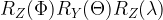
which is denoted by

in OpenQASM and Qiskit. For instance, 

Other gates can then be built from this family of one qubit gates. When it comes to multi-qubit gates, the only multi-qubit gate specified by OpenQASM is the CNOT gate denoted by CX, which can then again be combined with other gates to obtain gates operating on three and more qubits.
For qiskit, the available gates are specified in QASM syntax in the file qelib1.inc (see https://github.com/Qiskit/qiskit-terra/blob/master/qiskit/qasm/libs/qelib1.inc). Note that global phases are suppressed, so if you carry out the calculations, you will sometimes find a difference in the (unimportant) global phase between the result of the calculation and the results in Qiskit.
There is a couple of gates that you will often use in your circuits and that are summarized in the following table.
| Gate | Description |
|---|---|
| X | Pauli X gate |
| Y | Pauli Y gate |
| Z | Pauli Z gate |
| S | Phase gate  |
| T | T gate  |
| CX | CNOT gate |
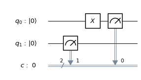
Gates take arguments that specify the qubits on which the gates operate. Individual qubits in a register can be addressed using an array-like notation. For example, to implement a circuit that applies an X gate to the first (least significant) qubit and then a controlled-NOT gate with this qubit as control qubit and the second qubit as target qubit, the following code can be used.
q = QuantumRegister(2,"q")
c = ClassicalRegister(2,"c")
circuit = QuantumCircuit(q,c)
circuit.x(q[0])
circuit.cx(q[0], q[1])
On real hardware, CNOTs can only be applied to specific combinations of qubits as specified in the coupling map of the device. However, when a circuit is prepared for execution on a specific device – a process called compilation – the compiler will deal with that by either reordering the qubits or adding additional swap operations.
Now we have gates, but to be able to run the circuit and measure the outputs, we still need measurements. These can easily been added with the measure method of a circuit, which accepts two parameters – the quantum register to measure and the corresponding classical register.
circuit.measure(q,c)
When the measurement step is reached during the processing of the circuit, the measurement is done – resulting in the projection of the state vector to the corresponding subspace – and the results of the measurements are copied into the classical register from which they can then be retrieved.
A nice property of Qiskit is its ability to visualize a quantum circuit. For that purpose, several classes called drawers are available in qiskit.tools.visualization. The circuit above, for instance, can be plotted with only one command
from qiskit.tools.visualization import matplotlib_circuit_drawer as drawer
my_style = {'cregbundle': True}
drawer(circuit, style=my_style)
and gives the nice representation
Compiling and running circuits
Let us now actually run the circuit. To do this, we need a Qiskit backend. Qiskit offers several backends. The Aer package contains a few simulators that are installed locally and can be executed directly from a Python script or a notebook. Some of these simulators calculate the actual state vectors (the unitary simulator and the state vector simulator), but cannot deal with measurements, others – the QASM simulator – only provide statistical results but can simulate the entire circuit including measurements.
The IBMQ package can be used to connect to the devices offered by the IBM Q experience program, including an online simulator with up to 32 qubits and the actual devices. As for the composer, accessing the IBM Q experience devices does obviously require an account and available units.
In order to run a circuit, we first compile the circuit, which will create a version of the circuit that is tailored for the specific hardware, and then submit the circuit as a job.
backend = IBMQ.get_backend('ibmq_16_melbourne')
from qiskit import compile
qobj = compile(circuit, backend=backend, shots=1024)
job = backend.run(qobj)
Once the job has been submitted, we can poll its status using job.status() every few seconds. When the job has completed, we can access the results using job.result(). Every job consists of a certain number of shots, i.e. individual executions, and the method result.get_counts() will return a hash map that lists the measured outcomes along with how often that outcome was obtained. The following gist shows a basic Python script that assembles a circuit, compiles it, submits a job to the Q experience and prints the results.
A few more features of the Qiskit package, including working with different simulators and visualization options as well as QASM output, are demonstrated in this script on my GitHub page. In one of the next posts, we will try to implement a real quantum algorithm, namely the Deutsch-Jozsa algorithm, and run it on IBMs device.
References
1. Andrew W. Cross, Lev S. Bishop, John A. Smolin, Jay M. Gambetta, Open Quantum Assembly Language, arXiv:1707.03429v2 [quant-ph]
2. The Qiskit tutorial on basic quantum operations
3. The Qiskit documentation

2 Comments