July 2018 – LeftAsExercise

First steps with Paperspace Gradient

So far, I have exclusively been using AWS EC2 when I needed access to a GPU – not because I have carefully compared the available offerings and taken a deliberate decision, but simply because I already had an EC2 account and know the platform.

However, I though it would be interesting to try out other platforms as well. In this post, I will talk a bit about my experience with Paperspace. This provider has several offerings – Core, which is basically an IaaS service, and Gradient, which allows you to access Jupyter notebooks and run jobs in ready-made environments optimized for Machine Learning – and of course I wanted to try this.

It should be noted that some time has passed between trying this out for the first time (roughly in May) and publication of this post in July, so bear with me when some of the details have changed in the meantime – Paperspace is still under development.

First steps

After signing up, you are routed to a page where you can choose between two products – Paperspace Core and Paperspace Gradient. I did choose Gradient (after providing the requested credit card information). The first thing I did try was to bring up a Jupyter notebook.

When you select that option, you have to make two choices. First, Jupyter notebooks are started in Docker containers, and you have to pick one of the available containers. Second, and more important, you have to select a machine – you have a choice between several CPU based and several GPU based models with different fees associated with them.

After a few seconds, your notebook is up and running (with the base account, you can only have one notebook server at any point in time). If you hit “Open”, a new tab will open and you will see the usual Jupyter home screen.

Your notebook folder will be prepopulated with some tutorials. The one I tried first is one of the classical MNIST / CNN tutorials. Unfortunately, when I tried to run it, the kernel died several times in a row – not very encouraging (it worked two days later, and overall there seem to be a few sporadic errors that come and go over time..).

Next, I could not resist the temptation to open a terminal. The Docker image seems to be based on a very basic Ubuntu distribution. I could successfully do an apt-get update && apt-get install git. So you could probably start to download things and work directly from the console – but of course this is not really the idea.

After playing for some time with the notebook, you can – again on the Paperspace notebook console stop your notebook (make sure to do this, you will be charged while the notebook is running). Once the notebook has stopped, you can click on the little arrow to the right of the notebook name, which will give you the option to download any files in the notebook directory that you have created in your session.

Once stopped, there is no way to restart a notebook, but you can clone a notebook which will create a copy of the previous notebook and start that copy, so you can continue to work where you left off. This works, but is a bit tiresome as you have to delete the obsolete copy manually.

Jobs

The next thing I tried is to create a job. For that purpose, you will first have to install the Paperspace CLI which in turn requires node.js and npm. So here is what you need to do on Ubuntu:

$ cd ~
$ apt install nodejs
$ apt install npm
$ npm install paperspace-node
$ sudo ln -s /usr/bin/nodejs /usr/bin/node

This will create a directory node_modules in your home directory and within that directory, a directory .bin. To test the paperspace CLI, you can run a command like

$ ./node_modules/.bin/paperspace --version

Next, switch to an empty directory and in that directory, run

$ ~/node_modules/.bin/paperspace project init

This will initiate a new paperspace project, i.e. it will create a subdirectory .ps_project containing a JSON configuration file. Next, you need an API key that you can get on your Paperspace home page. The API key is an authentication token that is used by the API – store that number in a safe place.

Once we have that token, it is time to start our first job.

 ~/node_modules/.bin/paperspace jobs create --container Test-Container --command "nvidia-smi" --apiKey "xxxxx" --machineType K80

where xxxxx needs to be replaced by your API key. Instead of providing your API key with every command, you can also run

$ ~/node_modules/.bin/paperspace login

which will add your credentials to a file in the .paperspace directory in your home directory.

Essentially, what happens when you run a job is that the local directory and all its subdirectories will be zipped into a file, a container will be set up on a Paperspace server, the content of the ZIP file will be extracted into this container and the command that you have specified will execute.

You can now get a list of your processes and their status either on the Paperspace console, where you also have immediate access to the log output, or from the command line using

$ ~/node_modules/.bin/paperspace jobs list

At this point, I was again a bit disappointed – the job appears to be running and is even displayed in the web console, but when it completes, I get an error “503 – Service unavailable” and no log output is provided. I raised a request with the support, and roughly 2 hours later the submission suddenly worked – I have not yet found out whether the support has really done anything or whether a part of the infrastructure was really down at this point in time.

As a temporary workaround, I managed to run a job by redirecting error output and standard output to a file. For instance, to run the script KMeans.py, I did use

$ ~/node_modules/.bin/paperspace jobs create  --command "export MPLBACKEND=AGG ; python KMeans.py > /artifacts/log 2>&1" --machineType C2

Once the job is complete, you can download whatever it has added to the directory /artifacts using

$ ~/node_modules/.bin/paperspace jobs artifactsGet --jobId "js26y3pi6jk056"

where the job ID is the ID of the job and will be displayed by the create command. Finally, the command jobs destroy --jobId=... can be used to delete a job after execution.

So far, I have to admit that I am not so happy with what I have seen. I hit upon several issues in the standard setup, and when playing around, I found that it can take a long time for a job to be scheduled on a GPU (depending very much on the machine type – my impression was that for machine types for which Paperspace uses GCP, like K80 or P100, your job will run quickly, but for other types like GPU+ it can take a long time). In addition, as everything is running in a container, the initial steps in job can be time consuming. TensorFlow, for instance, is known to take longer when it is started the first time, and in a fresh container, every time is a first time, so you will see a significant startup time. This gets worse if you need to download data sets, as this will have to be repeated with every new run. It is apparently not yet possible to mount a permanent volume into your container to avoid this or to reuse a stopped container (update: as of July, Paperspace has announced that the /storage directory is a persistent storage available across notebooks and jobs, but I have not yet tried this).

But maybe this is a premature judgement, and I decided that I will still continue to try it out. In one of the next posts, I will present some more advanced features and in particular the Python API that Paperspace offers.

The EM algorithm and Gaussian mixture models – part II

In this post, I will discuss the general form of the EM algorithm to obtain a maximum likelihood estimator for a model with latent variables.

First, let us describe our model. We suppose that we are given some joint distribution of a random variable X (the observed variables) and and random variable Z (the latent variables) and are interested in maximizing the likelihood of an observed sample x of the visible variable X. We also assume that the joint distribution depends on a parameter $\Theta$ , in practice this could be weights, bias terms or any other parameters. To simplify things a bit, we will also assume that the latent variable is finite. Our aim is to maximize the log likelihood, which we can – under these assumptions – express as follows.

$\ln P(x |\Theta) = \ln \sum_z P(x,z | \Theta)$

Even if the joint distribution belongs to some exponential family, the fact that we need to consider the logarithm of the sum and not the sum of the logarithms makes this expression and its gradient difficult to calculate. So let us look for a different approach.

To do this, let us assume that we are given a value $\Theta$ of the parameter and let us try to understand how the likelihood changes if we pass from $\Theta$ to some other value $\Theta'$ . For that purpose, we introduce a term that is traditionally called Q and defined as follows (all this is a bit abstract, but will become clearer later when we do an example):

$Q(\Theta'; \Theta) = E \left[ \ln P(x,z | \Theta') | x, \Theta \right]$

That looks a bit complicated, so let me explain the notation a bit. We want to define a function Q that will be a function of the new parameter value $\Theta'$ . This function will, in addition, depend on the current value $\Theta$ which we consider as a parameter.

The right hand side is an expectation value. In fact, for each value of the visible variable x and the parameter $\Theta$ , we have a probability distribution on the space in which Z lives, given by the conditional probability of Z given x and $\Theta$ . Whenever we have a function depending on z, we can therefore form the expectation value as usual, i.e. as the weighted sum over all function values, weighted by the probability of z. In particular, we can do this for the function $\ln P(x,z | \Theta')$ of z. Thus the right hand side is, spelled out

$E \left[ \ln P(x,z | \Theta') | x, \Theta \right] = \sum_z \ln P(x,z | \Theta') P(z | x, \Theta)$

That is now again a sum of logarithms, not a logarithm of a sum, and we can hope to be able to deal with this much better.

This is nice, but so far we have only introduced a rather complicated additional object – what do we gain? It turns out that essentially, maxizing Q will effectively maximize the likelihood. Let us make this bold statement a bit more precise. Suppose we are able to iteratively maximize Q. Expressed formally, this would mean that we are able to find a sequence $\Theta^0, \Theta^1, \dots$ of parameters such that when passing from $\Theta^t$ to $\Theta^{t+1}$ , the value of Q does not decrease, i.e.

$Q(\Theta^{(t+1)};\Theta^{(t)}) \geq Q(\Theta^{(t)} ; \Theta^{(t)})$

Then this very same sequence will be a sequence of parameters for which the log-likelihood is non-decreasing as well, i.e.

$\ln P(x | \Theta^{(t+1)}) \geq \ln P(x | \Theta^{(t)})$

I will not include a proof for this in this post (the proof identifies the difference between any two subsequent steps as a Kullback-Leibler divergence and makes use of the fact that a Kullback-Leibler divergence is never negative, you can find a a proof in the references, in particular in [2], or in my more detailed notes on the EM algorithm and Gaussian mixture models, where I also briefly touch on convergence). Instead, let us try to understand how this can be used in practice.

Suppose that we have already constructed some parameter $\Theta^t$ . The algorithm then proceeds in two steps. First, we calculate Q as a function of the new parameter $\Theta^{t+1}$ . As Q is defined as an expectation value, this step is called the expectation step. Once we have that, we try to maximize Q, i.e. we try to find a value for the parameter $\Theta^{t+1}$ such that $Q(\Theta^{t+1}; \Theta^t)$ is maximized. This part of the algorithm is therefore called the maximization step. Then we start over, using $\Theta^{t+1}$ as new starting point. Thus the algorithm alternates between an expectation and a maximization step, leading to the name EM algorithm.

To see how this works in practice, let us now return to our original example – Gaussian mixtures. Here the parameter $\Theta$ is given by

$\Theta = (\mu, \pi, \Sigma)$

We consider a random variable X which has N components, each of which being a vector X_n in a d-dimensional space and corresponding to one sample vector (so in the language of machine learning, N will be our batch size). Similarly, Z consists of N components z_n which again are subject to the restriction that only one of the z_nk be different from zero. We assume that the joint representation of our model is given by

$P(x , z) = \prod_n \prod_k \pi_k^{z_{nk}}{\mathcal N} (x_n, \mu_k , \Sigma_k)^{z_{nk}}$

Now we need to compute Q. The calculation is a bit lengthy, and I will skip most of it here (you can find the details in the references or my notes for this post). To state the result, we have to introduce a quantity called responsibility which is defined as follows.

$r_{nk} = \frac{\pi_k {\mathcal N}(x_n ; \mu_k, \Sigma_k)} {\sum_{j} \pi_j {\mathcal N}(x_n ; \mu_j, \Sigma_j) }$

From this definition, is it clear that the responsibility is always between zero and one, and in fact is has an interpretation of a (conditional) probability that sample n belongs to cluster k. Note that the responsibility is a function of the model parameters $\mu, \pi$ and $\Sigma$ . Using this notation, we can now write down the result of calculating the Q function:

$Q(\Theta'; \Theta) = \sum_n \sum_k r_{nk} \ln \pi'_k + \sum_n \sum_k r_{nk} \ln {\mathcal N}(x ; \mu'_k, \Sigma'_k)$

where the responsibilities are calculated using the old parameter set $\Theta = (\mu, \pi, \Sigma)$ . For a fixed $\Theta$ , this is a function of the new parameters $\mu', \pi'$ and $\Sigma'$ , and we can now try to maximize this function with respect to these parameters. This calculation is not difficult, but again a bit tiresome (and requires the use of Lagrangian multipliers as there is a constraint on the $\pi_k$ ), and I again refer to my notes for the details. When the dust settles, we obtain three simple expressions. First, the new values for the cluster means are given by

$\mu'_k = \frac{\sum_n r_{nk} x_n}{\sum_n r_{nk}}$

This starts to look familiar – this is the same expression that we did obtain for the cluster centers for the k-means algorithm! In fact, if we arrange the r_nk as a matrix, the denominator is the sum across column k and the numerators is the weighted sum over all data points. However, there is one important difference – it is no longer true that given n, only one of the r_nk will be different from one. Instead, the r_nk are soft assignments that model the probability that the data point x_n belongs to cluster k.

To write down the expression for the new value of the covariance matrix, we again need a notation first. Set

$N_k = \sum_n r_{nk}$

which can be interpreted as the number of soft assignments of points to cluster k. With that notation, the new value for the covariance matrix is

$\Sigma'_k = \frac{1}{N_k} \sum_n r_{nk} (x_n - {\mu'}_k)(x_n - {\mu'}_k)^T$

Finally, we can use the method of Lagrange multipliers to maximize with respect to the weights $\pi_k$ (which always need to sum up to one), and again obtain a rather simple expression for the new value.

$\pi'_k = \frac{N_k}{N}$

Again, this is intuitively very appealing – the probability to be in cluster k is updated to be the number of points with a soft assignment to k divided by the total number of assignments

We now have all the ingredients in place to apply the algorithm in practice. Let us summarize how this will work. First, we start with some initial value for the parameters – the weights $\pi$ , the covariance matrices $\Sigma_k$ and the means $\mu_k$ – which could, for instance, be chosen randomly. Then, we calculate the responsibilities as above – essentially, this is the expectation step, as it amounts to finding Q.

In the M-step, we then use these responsibilities and the formulas above to calculate the new values of the weights, the means and the covariance matrix. This involves a few matrix operations, which can be nicely expressed by the operations provide by the numpy library.

In the example above, we have created two sets of 500 sample points from different Gaussian mixture distributions and then applied the k-means algorithm and the EM algorithm. In the top row, we see the results of running the k-means algorithm. The color indicates the result of the algorithm, the shape of the marker indicates the original cluster to which the point belongs. The bottom row displays the results of the EM algorithm, using the same pattern.

We see that while the first sample (diagrams on the left) can be clustered equally well by both algorithms, the k-means algorithm is not able to properly cluster the second sample (diagrams on the right), while the EM algorithm is still able to assign most of the points to the correct cluster.

If you want to run this yourself, you can – as always – find the source code on GitHub. When playing with the code and the parameters, you will notice that the results can differ substantially between two consecutive runs, this is due to the random choice of the initial parameters that have a huge impact on convergence (and sometimes the code will even fail because the covariance matrix can become singular, I have not yet fixed this). Using the switch --data=Iris, you can also apply the EM algorithm to the Iris data set (you need to have a copy of the Iris data file in the current working directory) and find again that the results vary significantly with different starting points.

The EM algorithm has the advantage of being very general, and can therefore be applied to a wide range of problems and not just Gaussian mixture models. A nice example is the Baum Welch algorithm for training Hidden Markov models which is actually an instance of the EM algorithm. The EM algorithm can even be applied to classical multi-layer feed forward networks, treating the hidden units as latent variables, see [3] for an overview and some results. So clearly this algorithm should be part of every Data Scientists toolbox.

References

1. C.M. Bishop, Pattern recognition and machine learning, Springer, New York 2006
2. A.P. Dempster, N.M. Laird, D.B. Rubin, Maximum likelihood from incomplete data via the EM-algorithm, Journ. Royal Stat. Soc. Series B. Vol. 39 No. 1 (1977), pp. 1-38
3. Shu-Kay Ng, G.J. McLachlan, Using the EM Algorithm to Train Neural Networks: Misconceptions and a New Algorithm for Multiclass Classification, IEEE Transaction on Neural Networks, Vol. 15, No. 3, May 2004

The EM algorithm and Gaussian mixture models – part I

In the last few posts on machine learning, we have looked in detail at restricted Boltzmann machines. RBMs are a prime example for unsupervised learning – they learn a given distribution and are able to extract features from a data set, without the need to label the data upfront.

However, there are of course many other, by now almost classical, algorithms for unsupervised learning. In this and the following posts, I will explain one of the most commonly applied algorithms in this field, namely the EM algorithm.

As a preparation, let us start with a very fundamental exercise – clustering. So suppose that we are given a data set which we suspect to consist of K clusters. We want to identify these clusters, i.e. to each point in the dataset, we want to assign the number of the cluster to which the point belongs.

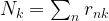
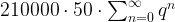
More precisely, let us suppose that we are given a set ${\mathcal D} = \{ x_i, \dots, x_N\}$ of points in some euclidian space and a number K of clusters. We want to identify the centre $\mu_i$ of each cluster and then assign the data points x_i to some of the $\mu_j$ , namely to the $\mu_j$ which is closest to x_i. We can encode the assignment of data points to clusters in a matrix R_ij where R_ij = 1 if data point x_i belongs to cluster j with centre $\mu_j$ . Thus each row of R corresponds to a data point and is non-zero in exactly one column, where it is one. This is known as 1-of-K encoding.

For each value of i, the squared distance of x_i to the centre of the cluster to which it is assigned is then given by

$\sum_j R_{ij} \| x_i - \mu_j |^2$

where we note that only one of the summands is different from zero. Assigning the data points to the clusters and positioning the centre points of the clusters then amounts to minimizing the loss function

$l(\mu, R) = \sum_i \sum_j R_{ij} \langle x_i - \mu_j , x_i - \mu_j \rangle$

where the brackets denote the usual euclidean scalar product.

Now let us see how we can optimize this function. For a fixed vector $\mu$ of cluster centers, we can easily minimize R_ij by assigning each data point to the cluster whose center is closest to x_i. Thus we set

$R_{ij} = \begin{cases} 1 & \text{if} \, j = \arg \min \| x_i - \mu_j \|^2 \\ 0 & \text{otherwise} \end{cases}$

Conversely, given a matrix R which we hold fixed, it is likewise easy to minimize $\mu_j$ . As there are no further constraints on $\mu_j$ , we can find the minimum by differentiating the loss function. We find that the derivative is zero if and only if

$0 = \sum_i R_{ij}(x_i - \mu_j)$

holds for all j. Assuming for a moment that each cluster has at least one data point assigned to it, i.e. that none of the columns of R contains zeroes only, we can solve this by

$\mu_j = \frac{\sum_i x_i R_{ij}}{\sum_i R_{ij}}$

which is also easily seen to be a local minimum by taking the second derivative.

Note that this term has an obvious geometric interpretation. The denominator in this expression is the number of data points that are currently assigned to cluster j. The numerator is the sum of all data points assigned to this cluster. Thus the minimum is the mean value of the positions of the data points that are currently assigned to the cluster (a physicist would call this the center of gravity of the cluster). This is the reason why this method is called the k-means algorithm. If no data points are assigned to the cluster, the loss function does not depend on $\mu_j$ and we can choose any value that we want.

The algorithm now works as follows. First, we choose centers $\mu_j$ at will – it is common to use some of the data points for this purpose. Then we assign each data point to a center using the formula for R_ij derived above. We then adjust the center points $\mu_j$ and reallocate the points to the new centers and so forth.

From our discussion above, it is clear that each full iteration of this procedure will reduce the loss function. This does of course not imply that the algorithm converges to a global minimum, as it might get stuck in local minima or saddle points. In practice, the algorithm is executed until the cluster assignments and centers do not change any more substantially or for a given number of steps.

The diagram above shows the result of applying this algorithm to a set of points that is organized in two clusters. To generate the data, 100 samples were drawn from 2-dimensional Gaussian distributions. On the left hand side, half of the the samples were centered at the point (5,1), the other samples at (1,4), and both had standard deviation 0.6. On the right hand side, the same centers were used, but only a small number of samples were drawn from the second distribution which had standard deviation 0.5, whereas most samples came from the first distribution with standard deviation 0.8. Then 10 iterations of the k-means algorithm were applied to the resulting sample set. The points in the sample were then plotted with a color indicating the assignment to clusters resulting from the matrix R. The actual cluster from which the sample was drawn is indicated by the shape – a point is cluster one, a diamond is cluster two.

We see that in the example on the left hand side, the algorithm has correctly assigned all points to their original cluster. For the example on the right hand side, the situation is different – the algorithm did actually assign significantly more points to the blue cluster, i.e. there are many wrong assignments (blue points). This does not change substantially if we increase the number of iterations, even with 100 iterations, we still see many wrong assigments for this example. If you want to reproduce the example and play a bit with the parameters, you can get the sourcecode for a straightforward implementation in Python from my GitHub repository.

The K-means algorithm is very simple and straightforward, but seems to have limitations because it cannot determine the shape of a distribution, only its center. It turns out that K-means is a special case of a broader class of algorithms that we now study, hoping to find more robust algorithms.

In our example, we have generated sample data as a combination of two Gaussian distributions. What if we just change the game and simply assume that our data is of this type? In other words, we assume an underlying probabilistic model for our sample data. Once we have that, we can pull all the tricks that statistical inference can offer – we can calculate maximum likelihood and maximum posterior probability, we can try to determine the posterior or even sample from the model.

Thus let us try to fit our data to a model of the form

$P(x) = \sum_k \pi_k {\mathcal N}(x ; \mu_k, \Sigma_k)$

where ${\mathcal N}(x ; \mu_k, \Sigma_k)$ is a multivariate Gaussian distribution with mean $\mu_k$ and covariance matrix $\Sigma_k$ , i.e.

${\mathcal N}(x ; \mu_k, \Sigma_k) = \frac{1}{\sqrt{(2\pi)^d \det(\Sigma)}} \exp (-\frac{1}{2} \langle x - \mu_k, \Sigma_k^{-1}(x - \mu_k)\rangle)$

and the $\pi_k$ are non-negative real numbers with $\sum_k \pi_k = 1$ .

Let us now see how this equation looks like if we use a 1-of-K encoding. We introduce a random variable Z that takes values in $\{ 0, 1\}^K$ with the additional constraint that only one of the Z_k is allowed to be different from zero. We interpret $\pi_k$ as the probability

$\pi_k = P(Z_k = 1)$

Then

$P(Z = z) = \prod_k \pi_k ^{z_k}$

and we can write

$P(X=x) = \sum_z P(Z=z) P(X=x | Z=z) = \sum_z P(x,z)$

where $P(z)$ is as above and

$P(X = x | Z = z) = \prod_k {\mathcal N}(x ; \mu_k, \Sigma_k)^{z_k}$

This is a very general type of distribution which reflects a common pattern in machine learning, namely the introduction of so called latent or hidden variables. In general, latent or hidden variables are random variables that are a part of the model which cannot be observed, i.e. are not part of the input or the output of the model. We have seen latent variables in action several times – adding hidden units to a neural network introduces latent variables and makes the model much more powerful, the hidden layer of a restricted Boltzmann machine serves as memory to learn features, and latent variables that are used to construct a mixture of Gaussians as above allow us to model a much broader class of distributions than a model with just one Gaussian.

Intuitively, it is also clear how to sample from such a model. In a first step, we sample from Z, in other words we determine the index k randomly according to the distribution given by the $\pi_k$ . Once we have k, we then sample from the conditional distribution $P(X = x | Z = z)$ . As we already have k, this amounts to sampling from the Gaussian distribution ${\mathcal N}(x ; \mu_k, \Sigma_k)$ with mean $\mu_k$ and covariance matrix $\Sigma_k$ .

In the example above, we have first applied this procedure to a one-dimensional Gaussian mixture with K=2. The histogram shows the result of the sampling procedure, the solid lines are the probability density functions of the two individual Gaussian distributions, multiplied by the respective weight. On the right hand side, the result of sampling a Gaussian mixture in two dimensions is displayed (you can download the notebook used to produce this example here).

When we now try to fit this model to the sample data, we again have to calculate the likelihood function and try to maximize it. However, it turns out that the gradient of the likelihood is not so easy to calculate, and it might very well be that there is no closed form solution or that we obtain rather complicated expressions for the gradient. Fortunately, there is an alternative that works for very general models and does not require knowledge of the gradient – the EM algorithm. In the next post, I will present the algorithm in this general setup, before we apply it to our original problem and compare the results with the k-means algorithm.

References

Controlling Docker container with Python

In the last few posts on the bitcoin blockchain, I have already extensively used Docker container to quickly set up test environments. However, it turned out to be a bit tiresome to run the containers, attach to them, execute commands etc. to get into a defined state. Time to learn how this can be automated easily using our beloved Python – thanks to the wonderful Docker Python SDK.

This package uses the Docker REST API and offers an intuitive object model to represent container, images, networks and so on. The API can be made available via a TCP port in the Docker configuration, but be very careful if you do this – everybody who has access to that port will have full control over your Docker engine. Fortunately, the Python package can also connect via the standard Unix domain socker on the file system which is not exposed to the outside world.

As always, you need to install the package first using

$ pip install docker

Let us now go through some objects and methods in the API one by one. At the end of the post, I will show how you a complete Python notebook that orchestrates the bitcoind container that we have used in our tests in the bitcoin series.

The first object we have to discuss is the client. Essentially, a client encapsulates a connection to the Docker engine. Creating a client with the default configuration is very easy.

import docker
client = docker.client.from_env()

The client object has only very few methods like client.info() or client.version() that return global status information. The more interesting part of this object are the collections attached to it. Let us start with images, which can be accessed via client.images. To retrieve a specific instance, we can use client.images.list(), passing as an argument a name or a filter. For instance, when we know that there is exactly one image called “alice:latest”, we can get a reference to it as follows.

alice = client.images.list("alice:latest")[0]

Other commands, like pull or push, are the equivalents of the corresponding docker CLI commands.

Let us now turn to the client.containers collection. Maybe the most important method that this collection offers is the run method. For instance, to run a container and capture its output, use

output = client.containers.run("alpine", "ls", auto_remove=True)

This will run a container based on the alpine image and pass “ls” as an argument (which will effectively execute ls as alpine container will run a shell for you) and return the output as a sequence of bytes. The container will be removed after execution is complete.

By setting detach=True, the container will run in detached mode and the call will return immediately. In this case, the returned object is not the output, but a reference to the created container which you can use later to work with the container. If, for instance, you wanted to start an instance of the alice container, you could do that using

alice = client.containers.run("alice:latest", auto_remove=True, detach=True)

You could then use the returned handle to inspect the logs (alice.logs()), to commit, to exec code in the container similar to the docker exec command (alice.exec_run) and so forth.

To demonstrate the possibilities that you have, let us look at an example. The following notebook will start two instances (alice, bob) of the bitcoin-alpine image that you hopefully have build when you have followed my series on bitcoin. It then uses the collection client.networks to figure out to which IP address on the bridge network bob is connected. Then, we attach to the alice container and run bitcoin-cli in this container to instruct the bitcoind to connect to the instance running in container bob.

We then use the bitcoin-cli running inside the container alice to move the blockchain into a defined state – we mine a few blocks, import a known private key into the wallet, transfer a certain amount to a defined address and mine a few additional blocks to confirm the transfer. Here is the notebook.

Sorry, something went wrong. Reload?

Sorry, we cannot display this file.

Sorry, this file is invalid so it cannot be displayed.

view raw DockerBitcoinSetup.ipynb hosted with ❤ by GitHub

Make sure to stop all containers again when you are done, it is comparatively easy to produce a large number of stopped containers if you are not careful and use this for automated tests. I usually run the container with the --rm flag on the command line or the auto_remove=True flag in Python to make sure that they are removed by the Docker engine automatically when they stop.

Of course nobody would use this to simply run a few docker containers with a defined network setup, there are much better tools like Docker Swarm or other container management solutions for this. However, the advantage of using the Python SDK is that we can interact with the containers, run commands, perform tests etc. And all this can be integrated nicely into integration tests using test fixtures, for instance those provided by pytest. A fixture could bring up the environment, could be defined on module level or test level depending on the context, and can add a finalizer to shut down the environment again after the test has been executed. This allows for a very flexible test setup and offers a wide range of options for automated testing.

This post could only give a very brief introduction into the Python Docker SDK and we will not at all discuss pytest and fixtures – but I invite you to browse the Docker SDK documentation and pytest fixtures and hope you enjoy to play with this!

How the number of bitcoins is limited

In some of the previous posts, we did already hit upon the file chainparams.cpp in the source code of the bitcoin reference client. It is interesting to go through this and understand the meaning of the various parameters defined there. One of them should catch your attention:

class CMainParams : public CChainParams {
public:
    CMainParams() {
        strNetworkID = "main";
        consensus.nSubsidyHalvingInterval = 210000;

What does this parameter mean? It is in fact not used awfully often, apart from some unit tests I could only locate it once, namely in validation.cpp.

CAmount GetBlockSubsidy(int nHeight, const Consensus::Params& consensusParams)
{
    int halvings = nHeight / consensusParams.nSubsidyHalvingInterval;
    // Force block reward to zero when right shift is undefined.
    if (halvings >= 64)
        return 0;

    CAmount nSubsidy = 50 * COIN;
    // Subsidy is cut in half every 210,000 blocks which will occur approximately every 4 years.
    nSubsidy >>= halvings;
    return nSubsidy;
}

The output of this function plays an important role when a new block is mined by mine.cpp – this is the amount (in Satoshis) that a miner earns in addition to the fees! Put differently, this is the amount of bitcoins that are created when a block is mined.

What this code tells us is that the amount of bitcoin added during mining starts with 50 and is divided by two every 210.000 blocks. So the amount of bitcoins mined is a given by the formula

$210000 \cdot 50 + 210000 \cdot 25 + 210000 \cdot 12.5 + \dots = \sum_{n=0}^\infty 210000 \cdot 50 \cdot \frac{1}{2}^n$

The mathematicians among us will recognize this as a geometric series

$210000 \cdot 50 \cdot \sum_{n=0}^\infty q^n$

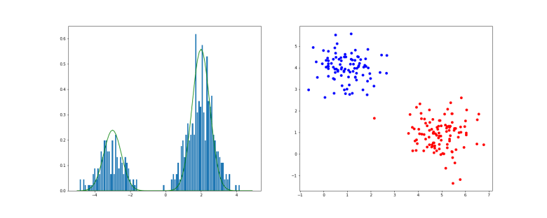
with $q = 0.5$ . This series converges, and its value is

$210000 \cdot 50 \cdot 2 = 21 \cdot 10^{6}$

Therefore the amount of bitcoins that are created by mining – and thus the overall supply of bitcoins – can never exceed roughly 21 million bitcoins. You might have heard that before: bitcoins are by designed with a controlled supply which is guaranteed by the continuous reduction of the subsidity as the number of blocks increases (and not because the value of a bitcoin transaction is stored in a 64 bit integer – in fact this would explain why the value of a single transaction output cannot exceed a certain value, but not why the total sum of all ever issued bitcoins is limited). This is the point in the source code that is responsible for this.

Of course I am cheating a bit – the value of a bitcoin is discrete, not a real number. Mining will stop if the value of the block subsidity falls below one Satoshi, as this is the smallest number that can be represented. Let us see when this happens. The subsidity is given by the formula

$s = \frac{5 \cdot 10^{9}}{2^n}$

where n is obtained by dividing the block height (i.e. length of the chain) by 210000 and converting to an integer. Solving $s = 1$ for n, we obtain

$n = \log_2 (5 \cdot 10^{9}) \approx 32.2$

Therefore the bitcoin amount created with a block will drop to zero with block

$m = 210000 * 33 = 6.930.000$ .

The total number of bitcoins created until then can be approximated (ignoring rounding) by the partial sum

$210000 \cdot 50 \cdot \sum_{n=0}^{32} q^n = \frac{50 \cdot 10^{9}(1 - q^{33})}{1 - q}$

which gives 20999999.997 bitcoins, i.e. almost exactly 21 million bitcoins as expected. We can also estimate when this will have happened. Looking at blockchain.info, we see that at the time of writing, approximately 513.000 blocks have already been mined. So we still need 6.418.000 blocks. A block is generated roughly every 10 minutes, so there are 6 additional blocks per hour and therefore 52560 blocks being added per year. Thus it will take roughly 122 years from now until all these blocks have been mined, i.e. this will happen somewhere around the year 2140. So still some time to go until then…

If you do not trust the math, you could also simulate this in a little Python program. In fact, this will give you a bit less than what we have calculated above, as the subsidity is rounded to an integer during the calculation, which our geometric series above does not properly reflect.

COIN = 10**8
nHeight = 0
btc = 0.0
while True:
    halvings = nHeight // 210000
    subsidity = (50*COIN) >> halvings
    btc += subsidity
    if subsidity < 1:
        break
    nHeight += 1

print("Total bitcoin amount: ", btc / 10**8 )

You can also easily determine how many bitcoin are available at each point in time. At 513.000 blocks, these are roughly 16.9 million BTC, which, at a price of 10.000 USD, is equivalent to a market capitalization of roughly 160 billion USD.