Navigating downhill: the quantum variational eigensolver

In quantum mechanics, the dynamics of a system is determined by its Hamiltonian, which is a hermitian operator acting on the Hilbert space that describes the system at hand. The eigenstates and eigenvalues of the Hamiltonian then correspond to stationary states and their energies, and finding these eigenstates and the corresponding eigenvalues is the central task in computational quantum mechanics.

Unfortunately, in most cases, this is very hard. First, the Hilbert space of most physically relevant systems is infinite-dimensional. However, even if we are able to approximate the Hamiltonian by a hermitian operator acting on a finite dimensional subspace, finding the eigenvalues and eigenstates by applying classical methods from numerical linear algebra like the QR method is computationally challenging due to the high dimensional spaces involved. It is natural to ask whether a quantum computer can help.

In fact, there are several methods available for finding eigenvalues of a hermitian matrix on a quantum computer. In 1995, A. Kitaev described an algorithm which is now known as the quantum phase estimation (see [2] and [3]) which can be used to estimate eigenvalues of unitary matrices (and can be applied to hermitian matrices as well noting that if A is a hermitian matrix, U = e^iAt is unitary and that there is an obvious relation between the eigenvalues of U and A). Unfortunately, this algorithm might require a large number (millions or even billions) of fault-tolerant quantum gates which is currently completely out of reach. This is the reason why a second algorithm which was first described in [1] and is designed to run on a quantum computer with a low number of qubits attracted a lot of attention. This algorithm, called the variational quantum eigensolver, might be able to deliver improvements over what is possible with classical hardware with somewhere between a few tens and one hundred qubits.

Setup and preliminaries

To explain the approach, let us assume that we are given a quantum register with n qubits and some hermitian operator H acting on the corresponding 2ⁿ-dimensional Hilbert space. We assume further that we can write our operator as a linear combination

$H = \sum_i h_i H_i$

of a small number of operators H_i which correspond to measurements that we can easily implement. An example could be a decomposition

$H = \sum_i h_i P_i$

where each P_i is a tensor product of Pauli matrices (it is not difficult to see that such a decomposition exists for every hermitian operator. First, write the operator as a linear combination of projections $|x_i \rangle \langle x_i |$ and the vectors as linear combinations of tensor products to show that each hermitian operator is a linear combination of tensor products of hermitian single-qubit operators, and then use the fact that each hermitian single qubit operator is a linear combination of Pauli matrices). A tensor product of Pauli matrices corresponds to a measurement that can be easily implemented by a combination of a measurement in the standard computational basis and a unitary transformation, see for instance this discussion of Pauli measurements.

Now if the operators H_i correspond to measurements that can efficiently be implemented, it is also possible to efficiently evaluate the expectation value

$\langle H_i \rangle = \frac{\langle \psi | H_i | \psi \rangle }{\langle \psi | \psi \rangle}$

for a given state $|\psi \rangle$ , assuming that we can efficiently prepare the state N times and then conduct N independent measurements – in fact, if N is sufficiently large, the expectation value will simply be the average over the measurements (see [4], section IV, for a more detailed discussion) – here we see a trade-off between the number of times we need to prepare the state $|\psi \rangle$ and measure and the resulting precision.

Once we are able to measure the expectation value of each H_i, we can easily obtain the expectation value of H as the weighted average

$\langle H \rangle = \sum h_i \langle H_i \rangle$

A second observation that we need in order to understand the variational quantum eigensolver is the fact that the problem of finding the eigenvalues can be reduced to a variational problem. In fact, suppose that we are given a hermitian matrix A on a finite dimensional Hilbert space with eigenvalues $\lambda_1, \lambda_2, \dots$ . Let us order the eigenvalues (which are of course real) such that $\lambda_1 \leq \lambda_2 \leq \dots$ , and let us assume that $|\psi_1 \rangle, |\psi_2 \rangle \dots$ is an orthonormal basis of corresponding eigenvectors.

If we are now given an arbitrary non-zero vector $|\psi \rangle$ , we can of course expand this vector as a linear combination

$|\psi \rangle = \sum_i a_i |\psi_i \rangle$

which immediately gives us the following expression for the expectation value

$\langle A \rangle = \frac{1}{\langle \psi | \psi \rangle} \sum_i |a_i|^2 \lambda_i$

Given the ordering of the eigenvalues, we can now estimate this number as follows.

$\langle A \rangle = \frac{1}{\langle \psi | \psi \rangle} \sum_i |a_i|^2 \lambda_i \geq \frac{1}{\langle \psi | \psi \rangle} \sum_i |a_i|^2 \lambda_1 = \lambda_1$

It is also obvious that we have equality if $|\psi \rangle$ is actually an eigenvector of A with eigenvalue $\lambda_1$ . Thus finding an eigenvector for the lowest eigenvalue of A is equivalent to minizing the expectation value of A!

This is at the heart of many variational methods like the Ritz method that have always been part of the toolset of computational quantum mechanics. In most of these methods, one considers state vectors parametrized by a finite dimensional parameter set, i.e. states of the form $|\psi(\Theta) \rangle$ where the parameter $\Theta$ ranges over some subset of a finite dimensional euclidian space. One then tries to minimize the expectation value

$\langle H \rangle (\Theta) = \frac{\langle \psi(\Theta) | H | \psi(\Theta) \rangle}{\langle \psi(\Theta) | \psi(\Theta) \rangle}$

using classical methods from mathematical optimization. The state vector minimizing this expectation value is then taken as an approximation for an eigenvector of H for its lowest eigenvalue.

Many classical optimiziation approaches that one might want to employ for this task work iteratively. We start with some value of the parameter $\Theta$ , then determine the expectation value, adjust the parameter, determine the next expectation value and so forth. Unfortunately, calculating the expectation value of a matrix in a high dimensional Hilbert space is computationally very hard, which makes this algorithm difficult to apply to quantum systems with more than a few particles.

The algorithm

This is the point where the quantum variational eigensolver comes into play. If the operator H can – as assumed above – be decomposed into a sum of operators for which finding the expectation value can efficiently be done, then we can efficiently determine the expectation value of H as well and can use that in combination with a classical optimization algorithm to find an approximate eigenvector for H.

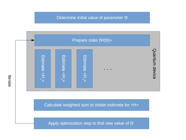
More precisely, here is the outline of the variational quantum eigensolver algorithm.

Decompose the operator H as a linear combination $H = \sum_\alpha h_\alpha H_\alpha$ where the expectation value of each $H_\alpha$ can be efficiently determined
Choose an initial value for the parameter $\Theta$
Prepare the quantum computer in the state $|\psi(\Theta) \rangle$
For each $H_\alpha$ , use measurements to determine the expectation value $\langle H_\alpha \rangle$
Calculate the expectation value of H as the weighted average $\langle H \rangle = \sum_\alpha h_\alpha \langle H_\alpha \rangle$
Apply a classical optimization step to determine a new value for the parameter $\Theta$
Start over with step 3 and repeat

So the algorithm switches forth and back between a quantum part – preparing the state and finding the expectation values – and a classical part, i.e. performing the actual optimization, and is therefore a prime example for a hybrid approach. This is visualized in the diagram below (which is a variation of the diagram presented in [1]).

Of course, to fully specify this algorithm, we have to define a method how to prepare the states efficiently and need to pick a classical optimization algorithm. In [1], the so-called coupled cluster method is chosen to prepare a state. In this method, the prepared state is given by applying a (parametrized) unitary transformation to a fixed reference state, and this unitary transformation can be efficiently implemented on a quantum computer. As an optimization algorithm, the downhill simplex method, also known as the Nelder-Mead method, is employed.

As noted in [1], the algorithm makes a certain trade-off between the number of iterations required to estimate the expectation values and perform the optimization step and the time required to run a single iteration on the quantum device. One of the main problems that todays quantum computers face, however, is to keep a quantum state stable over a longer period of time. Therefore the bottleneck is the run time or the number of operations that we spend in the quantum part of the algorithm, which this approach tries to minimize. As explained in [4], the variational principle also remains valid if we consider quantum systems with noise, which is an indication that the algorithm is comparatively resistant to noise. All this makes the quantum variational eigensolver a good candidate for a true quantum advantage on a near-term, noisy and not fully fault-tolerant quantum device.

Applications in computational chemistry

So far we have implicitly dealt with Hamiltonians H on a Hilbert space representing a quantum register, i.e. a tensor product of one qubit systems. For applications, there is therefore one additional step that we need to carry out in order to be able to apply the algorithm – we need to map the system and the Hamiltonian in question to an n-qubit quantum system. This involves in particular a projection of the (typically) infinite dimensional Hilbert space of the original problem onto a finite dimensional system.

A prime example that is detailed in [4] and in [1] is the Hamiltonian describing an atom with N electrons and their interactions with the nucleus and other electrons. Finding the eigenstates and eigenvalues of this Hamiltonian is known as the electronic structure problem.

In general, this is a difficult problem. Of course, the easiest case of this – the hydrogen atom – can be solved analytically and is treated in most beginner courses in quantum mechanics. However, already for the Helium atom, no closed solution is known and approximations have to be used.

In order to apply the variational quantum eigensolver to this problem, a mapping to a Hilbert space describing a quantum register needs to be done. As explained in [1], this can be done using the mechanism of second quantization and the Jordan-Wigner transform. In this paper, the authors have applied the method to estimate the strength of the chemical bond in a helium hydride ion HeH⁺, which is formed by the reaction of a proton with a helium atom. They show that in order to obtain a very good approximation, a four-dimensional Hilbert space is sufficient, so that the algorithm can be carried out on a quantum computer with only two qubits. Recently ([5]), this has been extended to a six-qubit system used to estimate the ground state energy of a BeH₂ molecule. Of course these are still comparatively small systems, but these experimental results encourage the hope that the approach scales and can be used on medium scale near-term quantum devices to go beyond what is possible with classical computers.

This work is also described in a post on the IBM website. IBM has made the Python sourcecode for similar applications available as part of its QISKit quantum computation library, so that everybody with a Q Experience account can run the algorithm and play with it. QISKit is a very interesting piece of software, and I will most likely devote one or more future posts on QISKit and similar frameworks like pyQUIL.

References

1. A. Peruzzo et. al., A variational eigenvalue solver on a photonic quantum processor, Nature Communications volume 5 (2014), available at www.nature.com/articles/ncomms5213
2. A. Kitaev, Quantum measurements and the Abelian Stabilizer Problem, arXiv:quant-ph/9511026
3. R. Cleve, A. Ekert, C. Macchiavello, M. Mosca, Quantum Algorithms Revisited, arXiv:quant-ph/9708016
4. J. R. McClean, J. Romero, R. Babbush, A. Aspuru-Guzik, The theory of variational hybrid quantum-classical algorithms, arXiv:1509.04279
5. A. Kandala, A. Mezzacapo, K. Temme,
M. Takita, M. Brink, J. M. Chow, J. M. Gambetta, Hardware-efficient Variational Quantum Eigensolver for Small Molecules and Quantum Magnets, Nature volume 549, pages 242–246 (14 September 2017), available as arXiv:1704.05018v2

Navigating downhill: the quantum variational eigensolver

Setup and preliminaries

The algorithm

Applications in computational chemistry

References

Published by christianb93

1 Comment

Leave a Comment Cancel reply

Setup and preliminaries

The algorithm

Applications in computational chemistry

References

Share this:

Like this:

Related

Published by christianb93

1 Comment

Leave a Comment Cancel reply