Mastering large language models – Part IX: self-attention with PyTorch

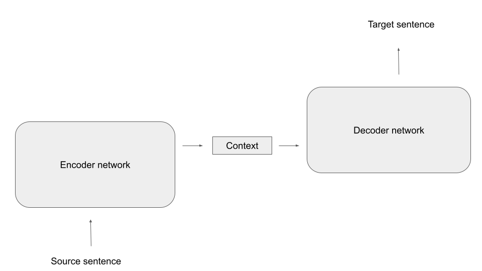
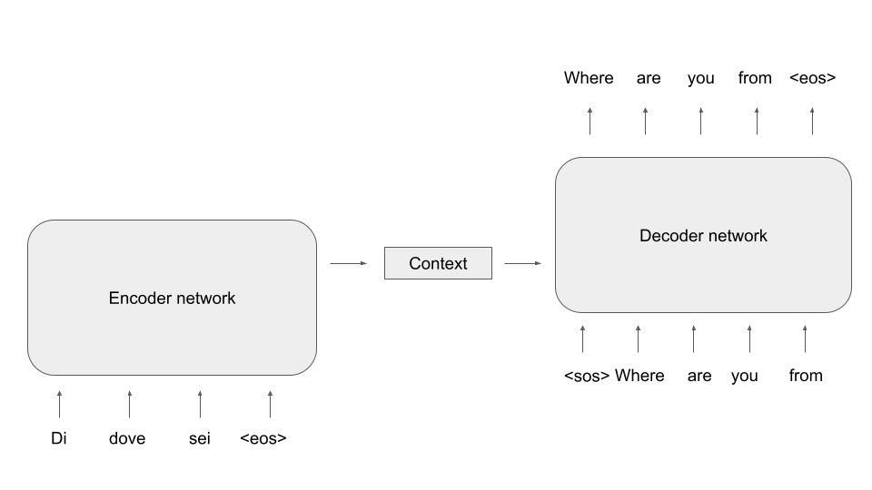
In the previous post, we have discussed how attention can be applied to avoid bottlenecks in encoder-decoder architectures. In transformer-based models, attention appears in different flavours, the most important being what is called self-attention – the topic of todays post. Code included.

Before getting into coding, let us first describe the attention mechanism presented in the previous blog in a bit more general setting and, along the way, introduce some terminology. Suppose that a neural network has access to a set of vectors vi that we call the values. The network is aiming to process the information contained in the vi in a certain context and, for that purpose, needs to condense the information specific to that context into a single vector. Suppose further that each vector vi is associated with a vector ki called the key, that somehow captures which information the vector vi contains. Finally assume that we are able to form a query vector q that specificies what information the network needs. The attention mechanism will then assemble a linear combination

\textrm{attn}(q, \{k_i\}, \{v_i\}) = \sum_i \alpha(q, k_i) v_i

called the attention vector.

To make this more tangible, let us look at an example. Suppose an encoder processes a sequence of words, represented by vectors xi. While encoding a part of the sentence, i.e. a specific vector, the network might want to pull in some data from other parts of the sentence. Here, the query would be the currently processed word, while keys and values would come from other parts of the same sentence. As keys, queries and values all come from the same sequence, this form of attention is called self-attention. Suppose, for example, that we are looking at the sentence (once again taken from “War and peace”)

The prince answered nothing, but she looked at him significantly, awaiting a reply

When the model is encoding this sentence, it might help to pull in the representation of the word “prince” when encoding “him”, as here, “him” refers to “the prince”. So while processing the token for “him”, the network might put together an attention vector focusing mostly on the token for “him” itself, but also on the token for “prince”.

In this example, we would compute keys and values from the input sequence, and the query would be computed from the word we are currently encoding, i.e. “him”. A weight is then calculated for each combination of key and query, and these weights are used to form the attention vector, as indicated in the diagram above (we will see in a minute how exactly this works).

Of course, this only helps if the weights that we use in that linear combination are somehow helping the network to focus on those values that are most relevant for the given key. At the same time, we want the weights to be non-negative and to sum up to one (see this paper for a more in-depth discussion of these properties of the attention weights which are a bit less obvious). The usual approach to realize this is to first define a scoring function

\textrm{score}(q, k_i)

and then obtain the attention weights as a softmax function applied to these scores, i.e. as

\alpha(q, k_i) = \frac{\exp(\textrm{score}(q, k_i))}{\sum_j \exp(\textrm{score}(q, k_j))}

For the scoring function itself, there are several options (see Effective Approaches to Attention-based Neural Machine Translation by Luong et al. for a comparison of some of them). Transformers typically use a form of attention called scaled dot product attention in which the scores are computed as

\textrm{score}(q, k) = \frac{q k^t}{\sqrt{d}}

i.e. as the dot product of query and key divided by the square root of the dimension d of the space in which queries and keys live.

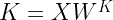
We have not yet explained how keys, values and queries are actually assembled. To do this and to get ready to show some code, let us again focus on self attention, i.e. queries, keys and values all come from the same sequence of vectors xi which, for simplicity, we combine into a single matrix X with shape (L, D), where L is the length of the input and D is the dimensionality of the model. Now the queries, keys and values are simply derived from the input X by applying a linear transformation, i.e. by a matrix multiplication, using a learnable set of matrices weights WQ (for the queries), WV (for the values) and WK (for the keys).

Q = X W^Q
K = X W^K
V = X W^V

Note that the individual value, key and query vectors are now the rows of the matrices V, K and Q. We can therefore conveniently calculate all the scaled dot products in one step by simply doing the matrix multiplication

\frac{Q \cdot K^T}{\sqrt{d}}

This gives us a matrix of dimensions (L, L) containing the scores. To calculate the attention vectors, we now still have to apply the softmax to this and multiply by the matrix V. So our final formula for the attention vectors (again obtained as rows of a matrix of shape (L, D)) is

\textrm{attn}(Q, K, V) = \textrm{softmax}\left(  \frac{Q \cdot K^T}{\sqrt{d}} \right) \cdot V

In PyTorch, this is actually rather easy to implement. Here is a piece of code that initializes weight matrices for keys, values and queries randomly and defines a forward function for a self-attention layer.

    
wq = torch.nn.Parameter(torch.randn(D, D))
wk = torch.nn.Parameter(torch.randn(D, D))
wv = torch.nn.Parameter(torch.randn(D, D))
    
#
# Receive input of shape L x D
#
def forward(X):
    Q = torch.matmul(X, wq)
    K = torch.matmul(X, wk)
    V = torch.matmul(X, wv)
    out = torch.matmul(Q, K.t()) / math.sqrt(float(D))
    out = torch.softmax(out, dim = 1)
    out = torch.matmul(out, V)
    return out
    

However, this is not yet quite the form of attention that is typically used in transformers – there is still a bit more to it. In fact, what we have seen so far is what is usually called an attention head – a single combination of keys, values and queries used to produce an attention vector. In real-world transformers, one typically uses several attention heads to allow the model to look for different patterns in the input. Going back to our example, there could be one attention head that learns how to model relations between a pronoun and the noun to which it refers. Other heads might focus on different syntactic or semantic aspects, like linking a verb to an object or a subject, or an adjective to the noun described by it. Let us now look at this multi-head attention.

The calculation of a multihead attention vector proceeds in three steps. First, we go through each of the heads which each has its own set of weight matrices (WQi, WKi, WVi) as before, and apply the ordinary attention mechanism that we have just seen to obtain a vector headi as attention vector for this head. Note that the dimension of this vector is typically not the model dimension D, but a head dimension dhead, so that the weight matrices now have shape (D, dhead). It is common, though not absolutely necessary, to choose the head dimension as the model dimension divided by the number of heads.

Next, we concatenate the output vectors of each head to form a vector of dimension nheads * dhead, where nheads is of course the number of heads. Finally, we now apply a linear transformation to this vector to obtain a vector of dimension D.

Here is a piece of Python code that implements multi-head attention as a PyTorch module. Note that here, we actually allow for two different head dimensions – the dimension of the value vector and the dimension of the key and query vectors.

class MultiHeadSelfAttention(torch.nn.Module):
    
    def __init__(self, D, kdim = None, vdim = None, heads = 1):
        super().__init__()
        self._D = D
        self._heads = heads
        self._kdim = kdim if kdim is not None else D // heads
        self._vdim = vdim if vdim is not None else D // heads
        for h in range(self._heads):
            wq_name = f"_wq_h{h}"
            wk_name = f"_wk_h{h}"
            wv_name = f"_wv_h{h}"
            wq = torch.randn(self._D, self._kdim)
            wk = torch.randn(self._D, self._kdim)
            wv = torch.randn(self._D, self._vdim)
            setattr(self, wq_name, torch.nn.Parameter(wq))
            setattr(self, wk_name, torch.nn.Parameter(wk))
            setattr(self, wv_name, torch.nn.Parameter(wv))
        wo = torch.randn(self._heads*self._vdim, self._D)
        self._wo = torch.nn.Parameter(wo)
        
    def forward(self, X):
        for h in range(self._heads):
            wq_name = f"_wq_h{h}"
            wk_name = f"_wk_h{h}"
            wv_name = f"_wv_h{h}"
            Q = X@getattr(self, wq_name)
            K = X@getattr(self, wk_name)
            V = X@getattr(self, wv_name)
            head = Q@K.t() / math.sqrt(float(self._kdim))
            head = torch.softmax(head, dim = -1)
            head = head@V
            if 0 == h:
                out = head
            else:
                out = torch.cat([out, head], dim = 1)
        return out@self._wo       

We will see in a minute that this implementation works, but the actual implementation in PyTorch is a bit different. To see why, let us count parameters. For each head, we have three weight matrices of dimensionality (D, dhead), giving us in total

3 x D x dhead x nheads

parameters. If the head dimension times the number of heads is equal to the model dimension, this implies that the number of parameters is in fact 3 x D x D and therefore the same as if we head a single attention head with dimension D. Thus, we can organize all weights into a single matrix of dimension (D, D), and this is what PyTorch does, which makes the calculation much more efficient (and is also better prepared to process batched input, which our simplified code is not able to do).

It is instructive to take a look at the implementation of multi-head attention in PyTorch to see what happens under the hood. Essentially, PyTorch reshuffles the weights a bit to treat the head as an additional batch dimension. If you want to learn more, you might want to take a look at this notebook in which I go through the code and also demonstrate how we can recover the weights of the individual heads from the parameters in a PyTorch attention layer.

If you actually do this, you might stumble upon an additional feature that we have ignored so far – the attention mask. Essentially, the attention mask allows you to forbid the model to look at certain parts of the input when processing other parts of the input. To see why this is needed, let us assume that we want to use attention in the input of a decoder. When we train the decoder with the usual teacher forcing method, we provide the full sentence in the target language to the model. However, we of course need to prevent the model from simply peaking ahead by looking at the next word, which is the target label for the currently processed word, otherwise training is trivially successful but the network has not learned anything useful.

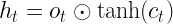
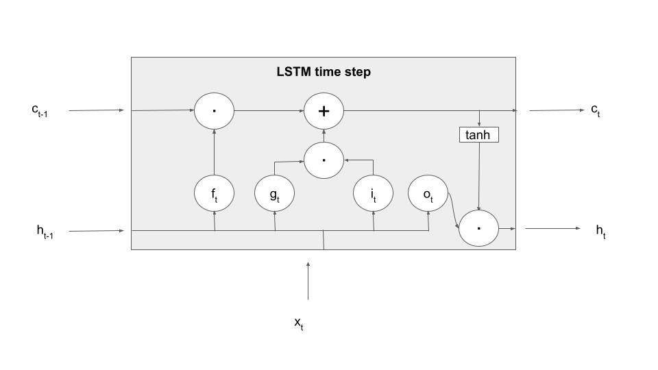
In an RNN, this is prevented by the architecture of the network, as in each time step, we only use the hidden state assembled from the previous time steps, plus the current input, so that network does not even have access to future parts of the sentence. In an attention-based model, however, the entire input is usually processed in parallel, so that the model could actually look at later words in the sentence. To solve this, we need to mask all words starting at position i + 1 when building the attention vector for word i, so that the model can only attend to words at positions less than or equal to i.

Technically, this is done by providing an additional matrix of dimension (L, L) as input to the self attention mechanism, called the attention mask. Let us denote this matrix by M. When the attention weights are computed, PyTorch does then not simply take the matrix product

Q \cdot K^T

but does in fact add the matrix M before applying the softmax, i.e. the softmax is applied to (a scaled version of)

Q \cdot K^T + M

To prevent the model from attending to future words, we can now use a matrix M which is zero on the diagonal and below, but minus infinity above the diagonal, i.e. for the case L = 4:

M = \begin{pmatrix} 0 & -\infty & -\infty & -\infty \\ 0 & 0 & -\infty & -\infty \\ 0 & 0 & 0 & -\infty \\ 0 & 0 & 0 & 0  \end{pmatrix}

As minus infinity plus any other floating point number is again minus infinity and the exponential in the softmax turns minus infinity into zero, this implies that the final weight matrix after applying the softmax is zero above the diagonal. This is exactly what we want, as it implies that the attention weights have the property

\alpha_{ij} = 0 \, \textrm{for } i < j

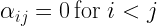
In other words, the attention vector for a word at position i is only assembled from this word itself and those to the left of it in the sentence. This type of attention mask is often called a causal attention mask and, in PyTorch, can easily be generated with the following code.

mask = torch.ones(L, L)
mask = torch.tril(mask*(-1)*float('inf'), diagonal = -1)
mask = mask.t()
print(mask)

This closes our post for today. We now understand attention, which is one of the major ingredients to a transformer model. In the next post, we will look at transformer blocks and explain how they are combined into encoder-decoder architectures.

Mastering large language models – Part VIII: encoder-decoder architectures and attention

The examples for LSTMs and RNNs that we have studied so far have one feature in common – the input and the output have the same length. We have seen that this is a natural choice for tasks like creating sentences based on a given prompt or attaching labels to each word in a sentence. There are, however, tasks for which this simple architecture cannot be used as we need to create a sentence based on an input of different length. To address this class of problems, encoder-decoder architectures have been developed which we will discuss today.

A good example to illustrate the challenge is machine translation. Here, we are given a source sequence, i.e. a sequence of token (x1, …, xS), maybe already vectorized, as input. The objective is to create a target sequence (y1, …, yT) as output representing the translation of the source sentence into a target language. Typically, the length T of the target sequence differs from the length S of the source sequence, which a single LSTM cannot easily cover.

Put differently, the objective is now no longer to model conditional probabilities for the completion of a sentence, i.e. probabilities of the form

P(w | w_1, \dots, w_n)

but conditional probabilities for a target sequence given the source sequence, i.e. the probability distribution

P(y_1, \dots, y_T | x_1, \dots, x_S)

The idea behind encoder-decoder architectures is to split this task into two subtasks, each of which is taken over by a dedicated network. First, there is a network called the encoder, that translates the source sequence into a single vector (or a concatentation of multiple vectors) called the context. The idea is that this vector represents, in a form independent of the length of the source sequence, an internal representation of the source sequence that somehow captures its meaning. Then a second network, the decoder, takes over. This network has access to the context and, given the context, creates the target sequence, as indicated in the diagram below..

In this general form, the idea is not bound to a specific type of network. Often, encoder and decoder are both LSTMs, but we will see in a later post that also transformer networks can be used in this way.

Let us now be a bit more specific on how we can bring this idea to live with LSTMs serving as decoders and encoders and specifically how these models are trained. For the encoder, this is easy – as we want the model to compress the meaning of the source sentence in the context, we of course need to feed the source sentence into the encoder. For the decoder, it is common to again apply teacher forcing. However, to create the first word of the target sentence, we need a starting point for the model. Therefore, the encoded sentences typically contain a “beginning of sentence” token, and it is also common practice to conclude the source sentence with a “end of sentence token”.

During inference, the model receives the source sequence as input and the first item of the target sequence, i.e. the beginning-of-sentence token. We can then apply any of the sampling methods discussed in an earlier post to successively generate the next word, until the model emits an end-of-sentence marker and the translation is complete.

Unfortunately, there is a fundamental problem with this architecture. If you look at the diagram, you will see that the context is the only connection between the encoder and the decoder. Consequently, the network has to compress all information necessary for the generation of the target sequence into the context, which is typically a vector of fixed size. Especially for longer source sentences, this quickly creates a bottleneck.

In 2015, Bahdanau, Cho and Bengio proposed a mechanism called attention to solve this issue. In their paper, they describe an approach which, instead of using a fixed-length context vector shared by all time steps of the decoder, uses a time-dependent context vector.

Specifically, each time step of the decoder receives three different inputs: the decoder input xt (which, as in the diagram above, is the previous word of the target sentence), the previous hidden state ht-1 and, in addition, a step-specific context ct. This context is assembled from the outputs os of the encoder network (these are in fact not exactly the hidden states, as the architecture proposed here uses a so-called bidirectional RNN as encoder, but let us ignore this for the time being). More precisely, each context vector ct is a weighted linear combination

c_t = \sum_s \alpha_{ts} o_s

of all outputs of the encoder network at all time steps. Thus, each decoder step has access to the full output of the encoder. However, and this is the crucial point, the way how the weights are calculated is governed by learned parameters which the network can adapt during training. This allows the decoder to focus on specific parts of the input sequence, depending on the current time step, i.e. to put more attention on specific time steps, lending the mechanism its name. Or, as the original paper puts it nicely in section 3.1:

The decoder decides parts of the source sentence to pay attention to. By letting the decoder have an attention mechanism, we relieve the encoder from the burden of having to encode all information in the source sentence into a fixed length vector.

To illustrate this, the authors include some examples for the weights used by the network. Let us look at the first of them, which illustrates the weights while translating the english sentence “The agreement on the European Economic Area was signed in 1992.”

We see that, as envisioned, the network learns to focus on the word that is currently being translated, even though the order of words in target and source sentence are different.

Attention turned out to be a very powerful idea. In fact, attention is so useful that it gave rise to a new class of language models which works without the need to have a hidden state which is updated sequentially over time. This new generation of networks is called transformers, and we will start to look at transformers and at attention scores in more detail in the next post.

References:

[1] Sequence to Sequence learning with Neural Networks, Sutskever et al.
[2] Learning Phrase Representations using RNN Encoder–Decoder for Statistical Machine Translation, Cho et al.
[3] Speech and Language Processing by Jurafsky and Martin, specifically chapter 9
[4] Neural Machine Translation and Sequence-to-sequence Models by Neubig
[5] Neural Machine Translation by Jointly Learning to Align and Translate, D. BahdanauK.ChoY. Bengio

Mastering large language models – Part VII: War and Peace

This blog is all about code – we will implement and train an LSTM on Tolstoys War and Peace and use it to generate new text snippets that (well, at least very remotely) resemble pieces from the original novel. All the code can be found here in my GitHub repository for this series.

First, let us talk about the data we are going to use. Fortunately, the original novel is freely available in a text-only format at Project Gutenberg. The text file in UTF-8 encoding contains roughly 3.3 million characters.

After downloading the book, we need to preprocess the data. The respective code is straightforward – we tokenize the text, build a vocabulary from the list of token and save the vocabulary on disk. We then encode the entire text and save 90% of the data in a training data set and 10% of the data in a validation data set.

The tokenizer requires some thoughts. We cannot simply use the standard english tokenizer that comes with PyTorch, as we want to split the text down to the level of the individual characters. In addition, we want to compress a sequence of multiple spaces into one, remove some special characters and replace line breaks by spaces. Finally, we convert the text into a list of characters. Here is the code for a simple tokenizer that does all this.

def tokenize(text):
    text = re.sub(r"[^A-Za-z0-9 \-\.;,\n\?!]", '', text)
    text = re.sub("\n+", " ", text)
    text = re.sub(" +", " ", text)
    return [_t for _t in text]

The preprocessing step creates three files that we will need later – train.json which contains the encoded training data in JSON format, val.json which contains the part of the text held back for validation and vocab.pt which is the vocabulary.

The next step is to assemble a dataset that loads the encoded book (either the training part or the validation part) from disk and returns the samples required for training. Teacher forcing is implemented in the __getitem__ method of the dataset by setting the targets to be the input shifted by one character to the right.

def __getitem__(self, i):
    if (i < self._len):
        x = self._encoded_book[i: i + self._window_size]
        y = self._encoded_book[i + 1: i + self._window_size + 1]
        return torch.tensor(x), torch.tensor(y)
    else:
        raise KeyError

For testing, it is useful to have an implementation of the dataset that uses only a small part of the data. This is implemented by an additional parameter limit that, if set, restricts the length of the dataset artificially to a given number of token.

Next let us take a look at our model. Nothing here should come as a surprise. We first use an embedding layer to convert the input (a sequence of indices) into a tensor. The actual network consists of an LSTM with four layers and an output layer which converts the data back from the hidden dimension to the vocabulary, as we have used it before. Here is the forward method of the model which again optionally accepts a previously computed hidden layer – the full model can be found here.

def forward(self, x, hidden = None):
    x = self._embedding(x) # shape is now (L, B, E)
    x, hidden = self._lstm(x, hidden) # shape (L, B, H)
    x = self._out(x)
    return x, hidden

Finally, we need a training loop. Training proceeds as in the examples we have seen before. After each epoch, we perform a validation run, record the validation loss and save a model checkpoint. Note, however, that training will take some time, even on a GPU – be prepared for up to an hour on an older GPU. In case you want to skip training, I have included a pretrained model checkpoint in the GitHub repository, so if you want to run the training yourself, remove this first. Assuming that you have set up your environment as described in the README, training therefore proceeds as follows.

cd warandpeace
python3 preprocess.py
# Remove existing model unless you want to pick up from previous model
rm -f model.pt
python3 train.py

Note that the training will look for an existing model model.pt on disk, so you can continue to train using a previously saved checkpoint. If you start the training from scratch and use the default parameters, you will have a validation loss of roughly 1.27 and a training loss of roughly 1.20 at the end of the last epoch. The training losses are saved into a file called losses.dat that you can display using GNUPlot if that is installed on your machine.

In case you want to reproduce the training but do not have access to a GPU, you can use this notebook in which I have put together the entire code for this post and run it in Google Colab, using one of the freely available GPUs. Training time will of course depend on the GPU that Google will assign to your runtime, for me training took roughly 30 minutes.

After training has completed (or in case you want to dive right away into inference using the pretrained model), we can now start to sample from the model.

python3 predict.py

The script has some parameters that you can use to select a sampling method (greedy search, temperature sampling, top-k sampling or top-p sampling), the parameters (temperature, k, p), the length of the sample and the prompt. Invoke the script with

python3 predict.py --help

to get a summary of the available parameters. Here are a few examples created with the standard settings and a length of 500 characters, using the model checked into the repository. Note that sampling is actually fast, even on a CPU, so you can try this also in case you are not working on a CUDA-enabled machine.

She went away and down the state of a sense of self-sacrifice. The officers who rode away and that the soldiers had been the front of the position of the room, and a smile he had been free to see the same time, as if they were struck with him. The ladies galloped over the shoulders and in a bare house. I should be passed about so that the old count struck him before. Having remembered that it was so down in his bridge and in the enemys expression of the footman and promised to reach the old…

Thats a wish to be a continued to be so since the princess in the middle of such thoughts of which it was all would be better. Seeing the beloved the contrary, and do not about that a soul of the water. The princess wished to start for his mother. He was the princess and the old colonel, but after she had been sent for him when they are not being felt at the ground of her face and little brilliant strength. The village of Napoleon was stronger difficult as he came to him and asked the account

Of course this is not even close to Tolstoy, but our model has learned quite a bit. It has learned to assemble characters into words, in fact all the words in the samples are valid english words. It has also learned that at the start of a sentence, words start with a capital letter. We even see some patterns that resemble grammar, like “Having remembered that” or “He was the princess”, which of course does not make too much sense, but is a combination of a pronoun, a verb and an object. Obviously our model is small and our training data set only consists of a few million token, but we start to see that this approach might take us somewhere. I encourage you to play with additional training runs or changed parameters like the number of layers or the model dimension to see how this affects the quality of the output.

In the next post, we will continue our journey through the history of language models and look at encoder-decoder architectures and the rise of attention mechanisms.

Mastering large language models – Part VI: sampling

Today, we will take a closer look at the process of using a trained LSTM or RNN to actually generate new content, i.e. to predict words. To set the scene, recall that the objective on which we have trained our network is to model the probability

P(w | w_1, \dots, w_n)

for each word in the vocabulary. More precisely, assume that our vocabulary has length V with elements v0, …, vV-1. Then the model is trained to predict for each i the probability that the next word is vi.

p_i = P(w = v_i| w_1, \dots, w_n)

As the network operates in time steps, it will create one corresponding vector p of probabilities with each time step, containing the probability distribution for the next word after having seen the input up to this point. Therefore the output of our model has shape (L, V), but we are only interested in the last output. In addition, recall that in practice, the softmax layer is usually not part of the model but contained in the loss function. Thus, to obtain the vector p of length V, we have to proceed as follows.

First, we take the sentence that we want to complete, the so-called prompt. We then tokenize this sentence and encode it as a tensor of shape L, where L is the number of token in the prompt. We feed this input vector x into the model and obtain the output (and the values of the hidden layer which we ignore). We then take the last element of the output and apply a softmax to obtain our probability distribution p. The corresponding code would look similar to this code snippet.

# x contains encoded prompt
f, _ = model(x)
 p = torch.softmax(f[-1], dim = 0)

which we have already seen in our toy model that was trained to complete a sequence of numbers. In this toy model, we have chosen the most straightforward approach to determine the next token from this probability distribution – take the index with the highest probability, i.e.

idx = torch.argmax(p).item()

This is again an index in our vocabulary. We can now look up the corresponding token in the vocabulary and append this token to our prompt. At this point, we have successfully extended the prompt by one generated token. We can now repeat the process to obtain a second token and so forth, until we have reached a certain specified minimum length. Note that in all steps but the first one, it is more efficient to feed the previously obtained hidden state back into the model, so that the model does not have to go through the entire sequence again. If we do this, however, we need to make sure that we feed only the last (just sampled) token as input, as the information on the previous part of the sentence is already encoded in the hidden state. Thus a complete function to sample could look as follows.

# Tokenize and encode prompt 
input_ids = [vocab[t] for t in tokenize(prompt)]
hidden = None
#
# Sample and append indices 
#
while (len(input_ids) < length):
    x = torch.tensor(input_ids, dtype = torch.long)
    x = x.to(device)
    #
    # Feed input ids into model
    #
    if hidden is None:
        f, hidden = model(x)
    else:
        f, hidden = model(x[-1].unsqueeze(dim = 0), hidden)
    #
    # f has shape (L, V) or (1,V) 
    # Take last element and apply softmax
    #
    p = torch.softmax(f[-1], dim = 0)
    #
    # Sample
    #
    idx = torch.argmax(p).item()
    #
    # and append   
    #
    input_ids.append(idx)

This will produce a list of indices which we still need to convert back into a string using the vocabulary.

The sampling method that we have applied here is sometimes called greedy sampling, because it greedily always selects the token with the highest probability weight. This is easy to implement (and fast), but has one major disadvantage – it is fully deterministic. Therefore the model easily gets stuck in loops during sampling and starts to repeat itself. This is in particular a problem if we use a short prompt, for instance “. ” to represent the start of a sentence. What we would actually want is a method that returns a reasonable sentence, but with some built-in randomness so that we do not always get the same sentence.

One way to do this is to actually draw a real sample from the probability distribution given by the vector p. PyTorch comes with a few helper classes to sample from various types of distributions, among them the categorical distribution which is actually nothing but a multinomial distribution. So instead of taking the argmax to determine the next index, we can use the line

idx = torch.distributions.categorical.Categorical(probs = p).sample()
idx = idx.item()

to draw an actual sample. Note that we first create a distribution object and then apply its sample method to perform the sampling. As the result is a tensor, we then use the item method to obtain a number that we can use as index into the vocabulary.

This sampling method is often applied with an additional parameter called the temperature. To understand this, let us discuss the impact of scaling the model output by some factor before applying the softmax. The softmax function is of course not linear, and due to the exponential function in the numerator, scaling by a large number will have a higher impact on those dimensions where the model output is already large. Thus scaling by a large number will increase existing spikes in the probability distribution. In the limit where the scaling factor tends to infinity, only the highest spike will survice and our sampling will be almost deterministic, so that we recover greedy search. Conversely, if the scaling factor is very small, the spikes will be softened, and eventually, in the limit when the scaling factor goes to zero, the resulting distribution will be the uniform distribution.

Traditionally, the parameter which is actually adjusted is the inverse of the scaling factor and is called the temperature. So the updated code including temperature looks like this.

# x contains encoded prompt
f, _ = model(x)
p = torch.softmax(f[-1] / temperature, dim = 0)

The discussion above shows that a small temperature value leads to a high scaling factor and therefore our sampling will become more and more deterministic, while a higher temperature will make the output more random (this is why the parameter is called the temperature, as this behaviour is what we also observe in statistical mechanics). Thus low temperatures are helpful if we want the model to stick as closely as possible to the training data, while higher temperatures make the model more creative. It is instructive to plot the probability distributions that different temperatures produce, I have done this in this notebook.

An extension of this sampling approach is known as top-k sampling (this method appears in Hierarchical Neural Story Generation by Fan et al., however, I am not sure whether this is really the first time this was proposed). In top-k sampling, we first pick the k indices with the highest probability weigths, were k is a parameter, rescale this to become a probability distribution again and sample from this modified distribution. The idea behind this is to avoid the tail distribution, i.e. to avoid that we accidentally sample very uncommon continuations, while still being more random than we are with greedy search. With PyTorch, this can be implemented as follows.

#
# Sort and remove all indices after the k-th index
#
_, indices = torch.sort(p, descending = True)
keep = indices[:k_val]
#
# Sample over the items that are left
#
_p = [p[i] for i in keep]
idx = torch.distributions.categorical.Categorical(probs = torch.tensor(_p)).sample()
idx = idx.item()
idx = keep[idx]        

Here we first use torch.sort to sort the probability distribution vector p in descending order, and then pick the k_val largest values, where k_val is the value of the k-parameter. So at this point, our array keep contains the indices that we want to sample from. We then collect the probabilities into a new probability vector and build a new multinomial distribution from this vector (which PyTorch will normalize automatically) from which we sample. As the output will be the position in the keep array, we still have to look up the actual index in this array.

Nucleus sampling or top-p sampling was proposed by Holtzman et al. in The curious case of neural text degeneration and extends this approach. Instead of using the k indices with the highest probability weights for a fixed value of k, we use those indices for which the total probability mass accounts for a certain minimum probability p_val, typically 0.9 or 0.95, i.e. we disregard the tail carrying the last 5% or 10% of the probability mass. The code is very similar, except that we first sum up the probabilities to determine the cut-off k and then proceed as for top-k sampling.

items , indices = torch.sort(p, descending = True)    
items = iter(items.tolist())
_sum = 0
_k = 0
while _sum <= p_val:
    _sum, _k =  _sum + next(items), _k + 1
keep = indices[:_k]
_p = [p[i] for i in keep]
idx = torch.distributions.categorical.Categorical(probs = torch.tensor(_p)).sample()
idx = idx.item()
idx = keep[idx]    

Of course, these methods can both be combined with a temperature parameter to control how creative the model can become. In practice, it is worth playing with different sampling methods and different values for the respective parameters (temperature, k, p) to see which combination gives the best results, depending on the use case.

We note that there is a family of sampling methods that we have not explained known as beam search, were instead of a candidate token, one tracks and scores candidates for entire sentences. Beam search is extensively described in the literature, for instance in Deep dive into deep learning section 10.8 or chapter 10 of Speech and Language Processing. Beam search can also be combined with sampling to obtain stochastic beam search. Finding the best method for sampling from large language models continues to be an active area of research. I encourage you to take a look at papers linked above, which provide a good overview of the various approaches to realize sampling and to measure the quality of the outcome.

This is a good point in time to look back at what we have discussed in the previous posts. We have learned how to tokenize a text, how to build a vocabulary and how to encode a text. We have then seen how various types of RNNs are implemented and trained, and finally we have looked at different methods to sample from the trained models. In the next post, we will put all this together and train a model on Tolstoys novel “War and peace”.

Mastering large language models – Part V: LSTM networks

In the last post, we have seen how we can implement and train an RNN on a very simple task – learning how to count. In the example, I have chosen a sequence length of L = 6. It is tempting to play around with this parameter to see what happens if we increase the sequence length.

In this notebook, I implemented a very simple measurement. I did create and train RNNs on a slightly different task – remembering the first element of a sequence. We can use the exact same code as in the last post and only change the line in the dataset which prepares the target to

 targets = torch.tensor(self._L*[index], dtype=torch.long)

I also changed the initialization approach compared to our previous post by using a random uniform distribution, similar to what PyTorch is doing. I then did training runs for different values of the sequence length, ranging from 4 to 20, and measured the accuracy on the training set after each training run.

The blue curve in the diagram below displays the result, showing the sequence length on the x-axis and the accuracy on the y-axis (we will get to the meaning of the upper curve in a second).

Clearly, the efficiency of the network decreases with larger sequence length, starting at a sequence length of approximately 10, and accuracy drops to less than 60%. I also repeated this with our custom build RNN replaced by PyTorchs RNN to rule out issues with my code, and got similar results.

This seems to indicate that there is a problem with higher sequence lengths in RNNs, and in fact there is one (you might want to take a look at this paper for a more thorough study, which, however, arrives at a similar result – RNNs have problems to learn dependencies in time series with a range of more than 10 or 12 time steps). Given that our task is to simply remember the first item, it appears that an RNNs memory is more of a short-term memory and less of a long term memory.

The upper, orange curve looks much more stable and maintains an accuracy of 100% even for long sequences, and in fact this curve has been generated using a more advanced network architecture called LSTM, which is the topic of todays post.

Before we explain LSTMs, let us try to develop an intuition what the problem is they are trying to solve. For that purpose, it helps to look at how backpropagation actually works for RNNs. Recall that in order to perform automatic differentiation, PyTorch (and similar frameworks) build a computational graph, starting at the inputs and weights and ending at the loss function. Now look at the forward function of our network again.

for t in range(L):
  h = torch.tanh(x[t] @ w_ih.t() + b_ih + h @ w_hh.t() + b_hh)
  out.append(h)

Notice the loop – in every iteration of the loop, we continue our calculation, using the values of the previous loop (the hidden layer!) as one of the inputs. Thus we do not create L independent computational graphs, but in fact one big computational graph. The depth of this graph grows with larger L, and this is where the problem comes from.

Roughly speaking, during backpropagation, we need to go back the entire graph, so that we move “backwards in time” as well, going back through all elements of the graph added during each loop iteration (this is why this procedure is sometimes called backpropagation in time). So the effective length of the computational graph corresponds to that of a deep neural network with L layers. And we therefore face one of the problems that these networks have – vanishing gradients.

In fact, when we run the backpropagation algorithm, we apply the chain rule at least once for every time step. The chain rule involves a multiplication by the derivative of the activation function. As these derivatives tend to be smaller than one, this can, in the worst case, imply that the gradient gets smaller and smaller with each time step, so that eventually the error signal vanishes and the network stops learning. This is the famous vanishing gradient problem (of course this is by no means a proof that this problem really occurs in our case, however, this is at least likely, as it disappears after switching to an LSTM, so let us just assume that this is really the case….).

So what is an LSTM? The key difference between an LSTM and an ordinary RNN is that in addition to the hidden state, there is a second element that allows the model to remember information across time steps called the memory cell c. At time t, the model has access to the hidden state from the previous time step and, in addition, to the memory cell content from the previous time step, and of course there is an input x[t] for the current time step, like a new word in our sequence. The model then produces a new hidden state, but also a new value for the memory cell at time t. So the new value of the hidden state and the new value of the cell are a function of the input and the previous values.

(h_t, c_t) = F(x_t, h_{t-1}, c_{t-1})

Here is a diagram that displays a single processing step of an LSTM – we fill in the details in the grey box in a minute.

So far this is not so different from an ordinary RNN, as the memory cell is treated similarly to a hidden layer. The key difference is that a memory cell is gated, which simply means that the cell is not directly connected to other parts of the network, but via learnable matrices which are called gates. These gates determine what content present in the cell is made available to the current time step (and thus subject to the flow of gradients during backward processing) and which information is kept back and used either not at all or during the next time step. Gates also control how new information, i.e. parts of the current input, are fed into the cells. In this sense, the memory cell acts a as more flexible memory, and the network can learn rules to erase data in the cell, add data to the cell or use data present in the cell.

Let us make this a bit more tangible by explaining the first processing step in an LSTM time step – forgetting information present in the cell. To realize this, an LSTM contains an additional set of weights and biases that allow it to determine what information to forget based on the current input and the previous value of the hidden layer, called (not surprisingly) the input-forget weight matrix Wif, the input-forget bias bif, and similarly for Whf and bhf. These matrices are then combined with inputs and hidden values and undergo a sigmoid activation to form a tensor known as the forget gate.

f_t = \sigma(W_{if} x_t  + b_{if} + W_{hf} h_{t-1} + b_{hf})

In the next step, this gate is multiplied element-wise with the value of the memory cell from the previous time step. Thus, if a dimension in the gate f is close to 1, this value will be taken over. If, however, a dimension is close to zero, the information in the memory cell will be set to zero, will therefore not be available in the upcoming calculation and in the output and will in that sense be forgotten once the time step completes. Thus the tensor f controls which information the memory cell is supposed to forget, explaining its name. Expressed as formula, we build

f_t \odot c_{t-1}

Let us add this information to our diagram, using the LaTex notation (a circle with a dot inside) to indicate the component-wise product of tensors, sometimes called the Hadamard-Product.

The next step of the calculation is to determine what is sometimes called the candidate cell, i.e. we want to select data derived from the input and the previous hidden layer that is added to the memory cell and thus remembered. Even though I find this a bit confusing I will instead follow the convention employed by PyTorch and other sources to use the letter g to denote this vector and call it the cell gate (the reason I find this confusing is that it is not exactly a gate, but, as we will see in a minute, input that is passed through the gate into the cell). This vector is computed similarly to the value of the hidden layer in an ordinary RNN, using again learnable weight matrices and bias vectors.

g_t = \tanh(W_{ig} x_t  + b_{ig} +  W_{hg} h_{t-1} + b_{hg})

However, this information is not directly taken over as next value of the memory cell. Instead, a second gate, the so-called input gate is applied. Then the result of this operation is added to the output of the forget gate times the previous cell value, so that the new cell value is now the combination of a part that survived the forget-gate, i.e. the part which the model remembers, and the part which was allowed into the memory cell as new memorizable content by the input gate. As a formula, this reads as

i_t = \sigma(W_{ii} x_t + b_{ii} + W_{hi} h_{t-1} + b_{hi})
c_t = f_t \odot c_{t-1} + i_t \odot g_t

Let us also update our diagram to reflect how the new value of the memory cell is computed.

We still have to determine the new value of the hidden layer. Again, there is a gate involved, this time the so-called output gate. This gate is applied to the value of the tanh activation function on the new memory cell value to form the output value, i.e.

o_t = \sigma(W_{io} x_t + b_{io} + W_{ho} h_{t-1} + b_{ho})
h_t = o_t \odot \tanh(c_t)

Adding this to our diagram now yields a complete picture of what happens in an LSTM processing step – note that, to make the terminology even more confusing, sometimes this entire box is also called an LSTM cell.

This sounds complicated, but actually an implementation in PyTorch is more straighforward than you might think. Here is a simple forward method for an LSTM. Note that in order to make the implementation more efficient, we combine the four matrices Wif, Wig, Wio and Wii into one matrix by concatenating them along the first dimension, so that we only have to multiply this large matrix by the input once, and similarly for the hidden layer. The convention that we use here is the same that PyTorch uses – the input gate weights come first, followed by the forget gate, than the cell gate and finally the output gate.,

def forward(x):    
    L = x.shape[0]
    hidden = torch.zeros(H)
    cells = torch.zeros(H)
    _hidden = []
    _cells = []
    for i in range(L):
        _x = x[i]
        #
        # multiply w_ih and w_hh by x and h and add biases
        # 
        A = w_ih @ _x 
        A = A + w_hh @ hidden 
        A = A + b_ih + b_hh
        #
        # The value of the forget gate is the second set of H rows of the result
        # with the sigmoid function applied
        #
        ft = torch.sigmoid(A[H:2*H])
        #
        # Similary for the other gates
        #
        it = torch.sigmoid(A[0:H])
        gt = torch.tanh(A[2*H:3*H])
        ot = torch.sigmoid(A[3*H:4*H])
        #
        # New value of cell
        # apply forget gate and add input gate times candidate cell
        #
        cells = ft * cells + it * gt
        #
        # new value of hidden layer is output gate times cell value
        #
        hidden = ot * torch.tanh(cells)
        #
        # append to lists
        #
        _cells.append(cells)
        _hidden.append(hidden)
    return torch.stack(_hidden)

In this notebook, I have implemented this (with a few tweaks that allow the processing of previous values of hidden layer and cell, as we have done it for RNNs) and verified that the implementation is correct by comparing the outputs with the outputs of the torch.nn.LSTM class which is the LSTM implementation that comes with PyTorch.

The good news it that even though LSTMs are more complicated than ordinary RNNs, the way they are used and trained is very much the same. You can see this nicely in the notebook that I have used to create the measurements presented above – using an LSTM instead of an RNN is simply a matter of changing one call, all the other parts of the data preparation, training loop and inference remain the same. This measurement also shows that LSTMs do in fact achieve a much better performance when it comes to detecting long-range dependencies in the data.

LSTMs were first proposed in this paper by Hochreiter and Schmidhuber in 1997. If you consult this paper, you will find that this original version did in fact not contain the forget gate, which was added by Gers, Schmidhuber and Cummins three years later. Over time, other versions of LSTM networks have been developed, like the GRU cell.

Also note that LSTM layers are often stacked on top of each other. In this architecture, the hidden state of an LSTM layer is not passed on directly to an output layer, but to a second LSTM layer, playing the role of the input from this layers point of view.

I hope that this post has given you an intuition for how LSTMs work. Even if our ambition is mainly to understand transformers, LSTMs are still relevant, as the architectures that we will meet when discussing transformers like encoder-decoder model and attention layers, and training methods like teacher forcing have been developed based on RNNs and LSTMs .

There is one last ingredient that we will need to start working on our first project – sampling, i.e. using the output of a neural network to create the next token or word in a sequence. So far, our approach to this has been a bit naive, as we just picked the token with the highest probability. In the next post, we will discuss more advanced methods to do this.