January 2019 – LeftAsExercise

Basics of quantum error correction

Do usable universal quantum computers exist today? If you follow the recent press releases, you might believe that the answer is “yes”, with IBM announcing a 50 qubit quantum computer and Google promoting its Bristlecone architecture with up to 72 qubits. Unfortunately, the world is more complicated than this – time to demystify the hype a bit.

The need for error correction

The important point is that it is not just the number of qubits that matters, but also their quality. When we study quantum algorithms like Shor’s algorithm, we are working with idealized qubits that behave exactly the way an isolated two-state quantum system is supposed to behave – these idealized qubits are often called logical qubits. However, in a real world implementation, there is no fully isolated two-state quantum system. Every system interacts to some extent with the environment, an interaction that we can try to reduce to a minimum, for instance by cooling our device down to very low temperatures, but never fully avoid. A trapped ion could, for instance, interact with radiation entering our device from the environment, and suddenly is part of a larger quantum system, consisting of the ion, the photons making up the radiation and maybe even the source of the photon. This will introduce errors into our system, i.e. deviations of the behavior of the system from the idealized theoretical model.

In addition to unwanted interactions with the environment, other errors could creep into our computation. When manipulating qubits to realize gates, we might make mistakes, for instance by directing a microwave pulse with a slightly incorrect frequency at our qubit, and we can make mistakes during each measurement.

Thus the real qubits in a quantum computer – called physical qubits – are prone to errors. These errors might be small for one qubit, but they tend to propagate through the circuit and add up to a significant error that will render the result of our quantum computation unusable. Thus we need error correction, i.e. the ability to detect and correct errors during our computation.

So how would you do this? Of course, errors can also occur in classical systems, and there are well developed methods to detect and correct them. Unfortunately, these approaches typically rely on the ability to copy and measure individual bits. This is easy for a classical bit, but more complicated for a qubit, as a measurement will collapse our system into an eigenstate of the observed operator and thus interfere with quantum algorithm.

The good news is that quantum error correction is still possible. In this post, I will try to explain the basics, before we then dive into more advanced topics in the next few posts.

Encoding logical states

In order to understand the basic ideas and structures behind quantum error correction, it is useful to study a simplified example – the three qubit code. To introduce this code, let us suppose that we have access to a communication channel across which we can send individual qubits from one quantum device to another one. Suppose further that this transmission is not perfect, but is subject to a bit flip error with a probability p. Thus, with probability p, a one-qubit state $|\psi \rangle$ will be changed to $X |\psi \rangle$ during transmission, where $X$ is the usual bit flip operator, and with probability 1-p, the transmission does not change the state. The aim is to construct an encoding of a qubit such that these errors can be detected and corrected.

To achieve this, we encode every single qubit state in a three-qubit state before transmitting it. Thus we use the following encoding

$|0 \rangle \mapsto |000 \rangle$

$|1 \rangle \mapsto |111 \rangle$

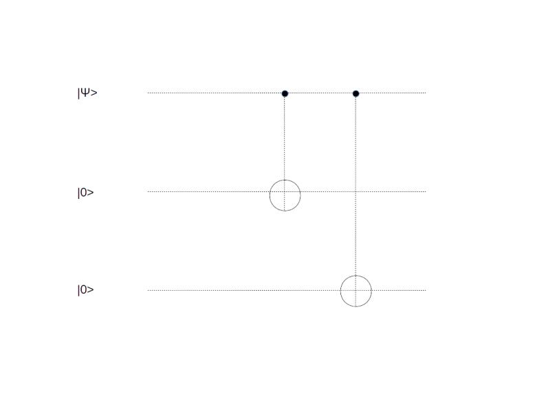
It is not difficult to see that this encoding can in fact be realized by a unitary circuit – the circuit below will do the trick.

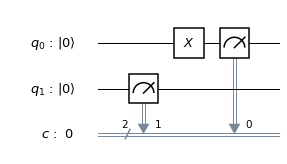
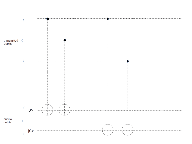
To transmit one qubit, we use this encoding to obtain a three-qubit message. We then send those three qubits through our communication channel. After the transmission, we apply a procedure known as syndrome measurement, using the following circuit.

Let us see what this circuit is doing. First, let us suppose that the original qubit was $|0 \rangle$ , encoded as $|000 \rangle$ , and no error did occur during the transmission. Then the three qubits at the top of the circuit will still be $|000 \rangle$ . In this case, the CNOT gates act as the identity, and the overall state after passing the circuit is

$|000 \rangle |00 \rangle$

Similarly, if the original qubit is $|1 \rangle$ and no error occurred, all CNOT gates will act as inversion. Thus the ancilla qubits will be inverted twice, and we end up with the state

$|111 \rangle |00 \rangle$

The situation is a bit different if a bit flip error has affected one of the qubits during the transmission, say the first one. Suppose the original state was again $|0 \rangle$ . After encoding and transmission with a bit flip on the first qubit, we will receive the state $|100 \rangle$ . Therefore both ancilla qubits will be inverted, and we obtain the state

$|100 \rangle |11 \rangle$

Let us now generalize these considerations. Assume that we are encoding the state $a |0 \rangle + b |1 \rangle$ , so that the encoded state will be $a |000 \rangle + b |111 \rangle$ . When we go through the above exercise for all possible cases, we arrive at the following table that shows the transmission error and the resulting state after passing the syndrome measurement circuit.

Error	Resulting state
No error	$(a \|000 \rangle + b \|111 \rangle ) \|00 \rangle$
Bit flip on first qubit	$(a \|100 \rangle + b \|011 \rangle ) \|11 \rangle$
Bit flip on second qubit	$(a \|010\rangle + b \|101 \rangle ) \|10 \rangle$
Bit flip on third qubit	$(a \|001\rangle + b \|110 \rangle ) \|01 \rangle$

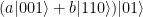
Now let us see what happens if we measure the ancilla qubits. First, note that all the states are already eigenstates for the corresponding measurement operator. Thus measuring the ancilla qubits will not change the state of the first three qubits and it will not reveal any information on the encoded state. The second important observation is that the value of the ancilla qubits tells us the exact error that has occurred. Thus we have found a way to not only find out that an error has occurred without destroying our superposition, but also to figure out which qubit was flipped. Given that information, we can now apply a bit flip operator once more to the affected qubit to correct the error. Again, this will not reveal the values of a and b and not collapse our state, and we can therefore continue to work with the encoded quantum state, for instance by running it through the inverse of the encoding circuit to get our original state back.

More general error models

So what we have found so far is that it is possible, also in the quantum world, to detect and protect against pure bit flip errors without destroying the superposition. But there is more we can learn from that example. In fact, let us revisit our original assumption that the only thing that can go wrong is that the operator X is applied to some of the qubits and allow a more general operator. Suppose, for instance, that our error is represented by applying to at most one of our qubits the operator

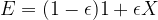
$E = (1-\epsilon) 1 + \epsilon X$

for a small $\epsilon$ . In contrast to our earlier assumption that the error operator is discrete, i.e. is either applied or not applied, this operator is now continuous, depending on the parameter $\epsilon$ , i.e. it looks as if we had to deal with a full continuous spectrum of errors. A short calculation shows that after transmitting and applying the syndrome measurement circuit above, the state of our quantum system will now be

Now let us again apply a measurement of the ancilla qubits. Then, according to the laws of quantum mechanics, the system will collapse onto an eigenstate, i.e. it will – up to normalization – end up in one of the states

$(\alpha |000 \rangle + \beta |111 \rangle)|00\rangle$

and

$(\alpha |100 \rangle + \beta |011\rangle) |11 \rangle$

But these are exactly the states in which we end up if no error occurs or a single bit flip error occurs. Thus, our measurement forces the system to somehow decide whether an error occurred or not and if yes, which error occurred – we are opening the box in which Schrödingers cat is hidden. This is a very important observation often referred to as the digitization of errors – it suffices to protect against discrete errors as the syndrome measurement will collapse any superposition of different errors states.

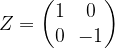
So far we have worked with a code which is able to protect against a bit flip error. But of course this is not the only type of error that can occur. At the first glance, it looks like there is a vast universe of potential errors that we have to account for, as in theory, the error could be any unitary operator. However, using arguments similar to the discussion in the last paragraph, one can show that it suffices to protect against two types of errors: the bit flip error discussed above and the phase flip error, represented by the matrix

$Z = \begin{pmatrix} 1 & 0 \\ 0 & -1 \end{pmatrix}$

Note that the phase flip error has no classical equivalent, other than the bit flip error which can classically be interpreted as a bit flipping from one to zero or vice versa randomly. The first error correction code that was able to handle both, bit flip errors and phase flip errors (and combinations thereof, ), and therefore any possible type of error (as long as the number of errors is limited) was described in 1995 by P. Shor. This code uses nine qubits to encode one logical qubit and is somehow a repeated application of the three bit code, based on the observation that the Hadamard transform turns a bit flip error into a phase flip error and vice versa. Later, different types of codes were discovered that are also universal in the sense that they protect against any potential one qubit error, i.e. against any error that only affects one qubit.

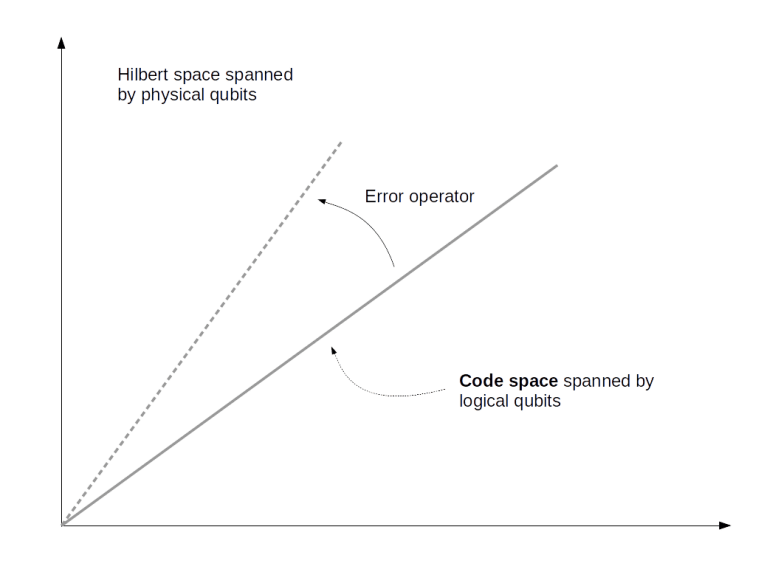
Let us now look at the structure that these codes have in common. First, the encoding can be described as identifying a 2-dimensional subspace C, called the code space, in the larger space spanned by all qubits. In the case of the three qubit code, the code space is spanned by the states $|000 \rangle$ and $|111 \rangle$ , corresponding to a logical zero and a logical one. More generally, the space C can have dimension 2ⁿ and the full Hilbert space can have dimension 2^k, in which case we can encode n qubits in a larger set of k qubits (in the nine qubit code example, k = 9 and n = 1).

Hence the code space is spanned by a set of 2ⁿ basis vectors $|\psi_i \rangle$ that we call code words. In the case n = 1, it is common practice to denote the codewords by $|0 \rangle_L$ and $|1 \rangle_L$ to indicate that they represent a logical qubit encoded using k physical qubits.

In addition, there is a set of error operators, i.e. a finite set of operators $\{ E_\alpha\}$ like the phase flip or bit flip operators acting on the larger Hilbert space. These operators represent the impact of discretized noise and will generally move the code words out of the code space, i.e. they will rotate the code space onto different subspaces of the entire Hilbert space.

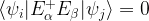
In order for a code to be useful, we of course need a relation between code space and errors that tells us that the errors can be detected and corrected. What are these conditions? A first condition is that no matter which errors occur, we can still tell the code words apart. This is guaranteed if the various error operators map different code words onto mutually orthogonal subspaces, in other words if

$\langle \psi_i | E_\alpha^{+} E_\beta | \psi_j \rangle = 0$

whenever $i \neq j$ and for all $\alpha, \beta$ . Thus, even in the presence of errors, the different code words will never overlap.

What about the case that both code words are the same? It is tempting to ask for the condition

$\langle \psi_i | E_\alpha^{+} E_\beta | \psi_i \rangle = \delta_{\alpha \beta}$

i.e. to require that different errors map the same codeword to orthogonal subspaces. This would make recovery very easy. We could perform the measurements that correspond to projections onto these subspaces to detect the error and correct them by applying the inverse of the error operator. However, this condition is too restrictive. In the case of the nine qubit code, for example, it might very well happen that two different errors map a code word to the same state. However, the same applies for the correction, i.e. we do not have to distinguish between these two errors as the act similarly on the code space. Therefore, a more general condition is usually used which captures this case:

$\langle \psi_i | E_\alpha^{+}E_\beta | \psi_j \rangle = C_{\alpha\beta} \delta_{ij}$

for a hermitian matrix $C_{\alpha \beta}$ . If the matrix has full rank, the code is called non-degenerate, otherwise – as in the case of the nine qubit code – the code is called degenerate.

Of course this encoding generates some overhead. To represent one logical qubit, we need more than one physical qubit. For the Shor code, we have to use nine physical qubits to encode one logical qubit. It is natural to ask what the minimum overhead is that we need. In 1996, Steane discovered a code that requires only seven physical qubits. In the same year, a code that requires only five qubits was presented and it was shown that this is a lower bound, i.e. there is no error correction code that requires less than five qubits.

So there is an unavoidable overhead – and the situation is even worse. To implement error correction, you need again quantum gates, which can of course also experience errors. Thus you need additional circuitry to protect the error correction against errors, which can again introduce errors and so forth. That there is a way out of this vicious circle is not obvious and the content of the famous threshold theorem that we will study in a later post – but even this way out is very hard to implement and might require thousands of physical qubits to implement one single logical qubit.

So even with a 72 qubit device, we are still far away from implementing only one logical qubit – and having a few thousand logical qubits to use Short’s algorithm to break an RSA key with a realistic key length is yet another story. So it is probably a good idea to take claims about universal supremacy of quantum computing within a few years with a grain of salt.

In this post, we have looked at some of the essential ideas behind quantum error correction, i.e. the ability to detect and correct errors. However, this is not enough to build a reliable quantum computer – after all, adding an error correction circuit introduces additional qubits that can also create new errors. In addition, we need to be able to perform calculations on our encoded states. So there is more that we need for fault-tolerant quantum computing which is the topic of the next post.

Using Python to access IBMs quantum computers

In a previous post, we have looked at IBMs Q experience and the graphical composer that you can use to build simple circuits and run them on the IBM hardware. Alternatively, the quantum hardware can be addressed using an API and a Python library called Qiskit which we investigate in this post.

Installation and setup

To be able to use Qiskit, there are some setup steps that we need to complete. First, we obviously have to install Qiskit. This is easy – we can simply use pip.

pip install qiskit

This will download the latest version of Qiskit, in my case (at the time of writing this) this was version 0.6.1. The next thing that you need is an API token to be able to access the IBM API. Assuming that you are already a registered user, you can create your token on the advanced tab of your user profile page.

In order to easily access your token from a Python script, it is useful to store the token locally on your hard drive. Qiskit uses a file qiskitrc in the ~/.qiskit folder in your home directory to store your credentials. The easiest way to create this file is the following code snippet

python -c 'from qiskit import IBMQ ; IBMQ.save_account("your_token")'

where obviously you need to replace the text inside the quotes with your token. After running this, you should find a file ~/.qiskit/qiskitrc containing your saved token (in clear text).

Once that file is in place, you can now easily load the credentials from within a Python program using the following code snippet

from qiskit import IBMQ
IBMQ.load_accounts()

The method IBMQ.active_accounts() will also return a list of currently available accounts which can be useful for debugging purposes. Loading an account is only needed if we want to connect to the IBM site to use their quantum hardware or the online simulator, not if we use a local backend – more on this later.

Circuits, gates and measurements

Let us now take a look at the basic data structures of Qiskit. A QuantumCircuit is what you expect – a collection of gates and registers. In Qiskit, a circuit operates on a QuantumRegister and optionally contains a ClassicalRegister which holds the results of a measurement. The following code snippet will create a quantum register with two qubits, a classical register with two qubits and a quantum circuit based on those registers.

from qiskit import QuantumCircuit
from qiskit import ClassicalRegister
from qiskit import QuantumRegister
q = QuantumRegister(2,"q")
c = ClassicalRegister(2,"c")
circuit = QuantumCircuit(q,c)

Next, we need to add gates to our circuit. Adding gates is done by calling the appropriate methods of the circuit object. The gate model of Qiskit is based on the OpenQASM language described in [1].

First, there are one qubit gates. The basic one qubit gates are rotations, defined as usual, for instance

$R_X(\Theta) = \exp \left( -i \frac{\Theta}{2} \sigma_X \right) = \cos \frac{\Theta}{2} - i \sigma_X \sin \frac{\Theta}{2}$

and similarly for the other Pauli matrices. Now it is well known that any rotation of the Bloch sphere can be written as a product of three rotations around y- and z-axis, i.e. in the form

$R_Z(\Phi)R_Y(\Theta)R_Z(\lambda)$

which is denoted by

$U(\Theta,\Phi,\lambda)$

in OpenQASM and Qiskit. For instance, $U(0, 0, \lambda)$ is a rotation around the z-axis and so forth. A short calculation shows that

$U(\Theta,\Phi,\lambda) = \begin{pmatrix} \exp \left(-\frac{i}{2}(\Phi + \lambda)\right) \cos \frac{\Theta}{2} & - \exp \left(-\frac{i}{2}(\Phi - \lambda)\right) \sin \frac{\Theta}{2} \\ \exp \left(\frac{i}{2}(\Phi - \lambda)\right) \sin \frac{\Theta}{2} & \exp \left(\frac{i}{2}(\Phi + \lambda)\right) \cos \frac{\Theta}{2} \end{pmatrix}$

Other gates can then be built from this family of one qubit gates. When it comes to multi-qubit gates, the only multi-qubit gate specified by OpenQASM is the CNOT gate denoted by CX, which can then again be combined with other gates to obtain gates operating on three and more qubits.

For qiskit, the available gates are specified in QASM syntax in the file qelib1.inc (see https://github.com/Qiskit/qiskit-terra/blob/master/qiskit/qasm/libs/qelib1.inc). Note that global phases are suppressed, so if you carry out the calculations, you will sometimes find a difference in the (unimportant) global phase between the result of the calculation and the results in Qiskit.

There is a couple of gates that you will often use in your circuits and that are summarized in the following table.

Gate	Description
X	Pauli X gate
Y	Pauli Y gate
Z	Pauli Z gate
S	Phase gate $\text{diag}(1,i)$
T	T gate $\text{diag}(1,e^{i\frac{\pi}{4}})$
CX	CNOT gate

Gates take arguments that specify the qubits on which the gates operate. Individual qubits in a register can be addressed using an array-like notation. For example, to implement a circuit that applies an X gate to the first (least significant) qubit and then a controlled-NOT gate with this qubit as control qubit and the second qubit as target qubit, the following code can be used.

q = QuantumRegister(2,"q")
c = ClassicalRegister(2,"c")
circuit = QuantumCircuit(q,c)
circuit.x(q[0])
circuit.cx(q[0], q[1])

On real hardware, CNOTs can only be applied to specific combinations of qubits as specified in the coupling map of the device. However, when a circuit is prepared for execution on a specific device – a process called compilation – the compiler will deal with that by either reordering the qubits or adding additional swap operations.

Now we have gates, but to be able to run the circuit and measure the outputs, we still need measurements. These can easily been added with the measure method of a circuit, which accepts two parameters – the quantum register to measure and the corresponding classical register.

circuit.measure(q,c)

When the measurement step is reached during the processing of the circuit, the measurement is done – resulting in the projection of the state vector to the corresponding subspace – and the results of the measurements are copied into the classical register from which they can then be retrieved.

A nice property of Qiskit is its ability to visualize a quantum circuit. For that purpose, several classes called drawers are available in qiskit.tools.visualization. The circuit above, for instance, can be plotted with only one command

from qiskit.tools.visualization import matplotlib_circuit_drawer as drawer
my_style = {'cregbundle': True}
drawer(circuit, style=my_style)

and gives the nice representation

Compiling and running circuits

Let us now actually run the circuit. To do this, we need a Qiskit backend. Qiskit offers several backends. The Aer package contains a few simulators that are installed locally and can be executed directly from a Python script or a notebook. Some of these simulators calculate the actual state vectors (the unitary simulator and the state vector simulator), but cannot deal with measurements, others – the QASM simulator – only provide statistical results but can simulate the entire circuit including measurements.

The IBMQ package can be used to connect to the devices offered by the IBM Q experience program, including an online simulator with up to 32 qubits and the actual devices. As for the composer, accessing the IBM Q experience devices does obviously require an account and available units.

In order to run a circuit, we first compile the circuit, which will create a version of the circuit that is tailored for the specific hardware, and then submit the circuit as a job.

backend = IBMQ.get_backend('ibmq_16_melbourne') 
from qiskit import compile
qobj = compile(circuit, backend=backend, shots=1024)
job = backend.run(qobj)

Once the job has been submitted, we can poll its status using job.status() every few seconds. When the job has completed, we can access the results using job.result(). Every job consists of a certain number of shots, i.e. individual executions, and the method result.get_counts() will return a hash map that lists the measured outcomes along with how often that outcome was obtained. The following gist shows a basic Python script that assembles a circuit, compiles it, submits a job to the Q experience and prints the results.

Sorry, something went wrong. Reload?

Sorry, we cannot display this file.

Sorry, this file is invalid so it cannot be displayed.

view raw QiskitSampleSubmission.ipynb hosted with ❤ by GitHub

A few more features of the Qiskit package, including working with different simulators and visualization options as well as QASM output, are demonstrated in this script on my GitHub page. In one of the next posts, we will try to implement a real quantum algorithm, namely the Deutsch-Jozsa algorithm, and run it on IBMs device.

References

1. Andrew W. Cross, Lev S. Bishop, John A. Smolin, Jay M. Gambetta, Open Quantum Assembly Language, arXiv:1707.03429v2 [quant-ph]
2. The Qiskit tutorial on basic quantum operations
3. The Qiskit documentation

Accessing your hard drive – the OS developers moment of truth

When building your own operating system, the moment when you first write data to a real physical hard disk of a real PC is nothing less than thrilling – after all, making a mistake at this point could mean that you happily overwrite data on your hard drive randomly and wipe out important data on your test machine.

So working with real hard drives is nothing for the faint of heart – but course, no operating system would be complete without that ability. In this post, we look at the basic concepts behind the communication between the operating system and the hard drive.

First, let us see how data on a hard drive is stored. The most basic conceivable hard drive consists of a thin disk, called a platter, on which the data is stored, and a device called head that is able to read and write data. The disk is spinning and the head can be moved forth and back across the disk, so that it can be positioned at an arbitrary distance from the center of the disk.

Physically, the disk is organized in concentric tracks. When the head is positioned at a certain distance from the center of the disk, it can therefore access an individual track. Tracks are further separated into sectors, as shown in the upper part of the diagram below (taken from this Wikipedia page). Finally, a block is the intersection of a sector with a track. So to identify a specific block, you could use the combination of a sector and the track on which the block is located.

This simple design is actually wasting some space, as you could only use one side of the disk. If you want to store data on both sides, you need two heads – one below and one above the disk. You could even increase the capacity further by building a stack of platters, which heads being located between the platters so that each side of a platter corresponds to one head reading from it and writing to it, as displayed in the lower part of the diagram.

In this setup, the union of tracks locates at corresponding positions on all platters is called a cylinder. If you know the cylinder and the head, you know the track. You could therefore specify the location of a block on the disk by the combination of a cylinder, a head and a sector. This addressing method is therefore called the CHS addressing and was the first addressing mode used on early IBM PCs and compatible machines.

Later, the actual geometry of the hard drive became more complicated, and addressing schemes that decouple the actual geometry of the hard drive from the address were introduced, most notably the so-called logical block addressing (LBA). In that addressing mode, which is the current standard, a hard disk is thought of as a sequence of blocks, numbered starting with zero. To access a block, you simply specify the number of the block. The hard disk controller, i.e the circuitry that is actually operating the hard drive and sitting between the CPU and the actual hard drive, will convert this LBA number into the actual physical location of the data on the drive.

So how do we actually access a block? The easiest way to do this is usually called programmed input output (PIO). To explain this, we first need to recall that a CPU is not only accessing the system memory, but can also talk to devices using designated channels, so called ports. If the CPU writes to a port, the data will be sent to the device, and vice versa data written by the device can be accessed by the CPU by reading from a port.

So to read from a hard drive, we could proceed as follows. First, we would write a command to a specific port associated with the hard drive. This command would tell the hard drive what to do – for instance to read – and it would contain the LBA number of the block we want to read. Then the hard drive controller would perform the actual read operation, and once complete, would send the data back to the CPU that would then read it from a port.

The format of the commands and the exact interaction between the CPU and the device in this process were defined in a standard called ATA, also called IDE or Parallel ATA (PATA). This specification did not only describe the interaction between the hard disk controller and the CPU, but also the low-level electronics, cables, connectors and so forth.

This method of reading and writing data is simple, but has a major disadvantage – it keeps the CPU busy. In the worst case, the CPU has to write the command, wait in a busy loop and then read the data one word at a time – and if you wanted to read several blocks, you had to do this over and over again. Not surprising that alternatives were developed soon.

The first improvement we can make is to make the operation interrupt driven. In this version, the CPU would send a command and could then go off and do something else while the hard disk controller is working. Once the data has been read, the controller informs the CPU that data is available by raising an interrupt, and the CPU can go ahead and fetch the data. This is already more efficient, but still suffers from the fact that the data has to be read byte for byte.

Consequently, the next step in the development was what is called Direct Memory Access (DMA). With DMA, the hard disk controller can communicate directly with the memory controller and transfer the data read directly into a designated area of the systems main memory without any involvement of the CPU. Only once all the data has been read, an interrupt is raised to raised to inform the CPU that the data has been transferred and can be worked with. With this approach, large blocks of data can be read and written while the CPU is able to work on other threads.

In 2000, a serial version of the ATA standard called Serial ATA (SATA) was introduced. Due to the serial processing, SATA allows much higher transfer rates between the hard drive and the motherboard and therefore a much higher I/O throughput and soon involved into the de-facto standard, also for consumer PCs. A SATA device can still operate in a so-called legacy mode, where it is presented to the CPU as a PATA/IDE device. However, to take advantages of some new features of the SATA protocol, for instance a higher number of devices per controller, a new protocol for the communication between the CPU and the controller needs to be used which is called AHCI. The AHCI protocol is significantly more complicated than the ATA protocol, but in fact both protocols still follow the same logical steps to read and write data.

Let us now combine this understanding with what we have learned about interrupts and multitasking to see how the operating system would typically orchestrate a disk drive access, for instance to read data from the disk. The following diagram illustrates the process.

First, the operating system reserves an area of system memory for the DMA transfer. Then, the kernel prepares the command. The format of the command depends on the used protocol (AHCI or legacy IDE), but typically, the command would encompass the location of the data on the disk to be read, the number of blocks to be read and the location of the DMA buffer. Then the command is sent to the hard drive.

At this point in time, the CPU is free to work on something else, so the kernel would typically put the current task to sleep and re-schedule so that a different task can start executing.

While this happens, the hard drive starts to execute the command. It reads the requested data and places it in the DMA buffer prepared by the OS. Then it raises an interrupt to indicate that the data has arrived in main memory.

Once the operating system receives the interrupt, it will stop the currently executing task and switch back to the task that requested the read. This task can now continue execution and work with the data.

Of course, the real picture is more complicated. What the image above calls the “device”, for instance, is in reality a combination of the actual hard disk controller and components of your motherboards chip set, like the AHCI controller or the DMA controller. In addition, several hard drives can operate in parallel, so the kernel needs a way to keep track of the currently executing requests and map incoming interrupts to the requests currently in flight. And, in an SMP environment with more than one CPU, semaphores or other locking mechanism need to be in place to make sure that different requests do not collide. If you are interested in all those details, you might want to take a look at the documentation of the ctOS hard disk driver.

We now understand how a hard drive and an operating system kernel communicate to read or write sectors. However, an application does of course not see individual blocks of a hard disk, instead the hard disk appears as a collection of files and directories. The translation between this logical view and the low-level view is done by the file system at which we will look in the next post in this series.

Quantum simulation

In his famous lecture Simulating Physics with computers, Nobel laureate Richard Feynman argued that non-trivial quantum systems cannot efficiently be simulated on a classical computer, but on a quantum computer – a claim which is widely considered to be one of the cornerstones in the development of quantum computing. Time to ask whether a universal quantum computer can deliver on that promise.

At the first glance, this seems to be obvious. Of course, there is one restriction – similar to classical computing, the resources of a quantum computer are finite, se we can only hope to be successful if we can at least approximately reduce the Hilbert space of the original problem to a finite dimensional space. But once this hurdle is taken, everything else looks easy. The time evolution of the system is governed by its Hamiltonian H – over a period of time t, the evolution of the system is described by the unitary operator

$U(t) = e^{iHt}$

This is a unitary operator, so given a universal set of quantum gates, we should – at least approximately – be able to implement this unitary evolution as a sequence of quantum gates. And we are able to store a state in a Hilbert space of dimension 2^N in N qubits, in contrast to the exponential number of classical bits that we would need. So what is the problem?

The problem is hidden in the complexity to construct an arbitrary unitary operator from a finite set of quantum gates. Suppose we are considering a quantum system with a finite number of qubits N so that a unitary operator is described by an 2^N x 2^N matrix. As argued in [1], if we assemble unitary operators from a set of universal gates, we need in the order of 2^2N steps, as this number of parameters is required to specify an arbitrary (binary) matrix of size N. Thus we have mastered the memory bottleneck only to run into a time bottleneck, as the number of steps still grows exponentially with the dimension of the Hilbert space.

In addition, figuring out how to build up the unitary matrix from the given set of universal gates – a task typically accomplished with a classical computer – can still be extremely difficult and scale exponentially with N. So it seems that we are fighting a lost battle (see also section 4.5.4 of [2] for an argument why building general unitary matrices from an elementary set of gates is hard).

Fortunately, this is only true if we insist on simulating any conceivable unitary matrix. In practice, however, most Hamiltonians are much simpler and built from local interactions – and this turns out to be the key to efficiency.

As an example to illustrate this point, let us consider a typical system of interest – a lattice in space that has a particle of spin 1/2 attached to each of its vertices. Suppose further that any particle only interacts with adjacent particles. Then, in the easiest case of constant coupling, the Hamiltonian of this system can be written as

$H = \sum_{\text{pairs} \, i,j} S_i S_j$

with spin operators S_i. The number of terms in the sum is proportional to N as we only allow pairs of adjacent spins to interact – actually it is roughly equal to 2N (each spin site pairs up with four other spins, and we need to divide by two as we double count – and there will be slight deviations from this rule depending on the boundary conditions). At every spin site, we have a two-dimensional Hilbert space describing that spin. If two sites i and j are adjacent, the operator S_iS_j acts on the tensor product of the Hilbert spaces attached to the involved sites, i.e. on a subspace of dimension four of the overall Hilbert space. The crucial point is that even though the dimension of the overall Hilbert space is huge, each term in the Hamiltonian only acts on a rather small subspace.

Let us now consider more general Hamiltonians of this form. Specifically, let us assume that we can write our Hamiltonian as a sum

$H = \sum_{s=1}^l H_s$

of l = 2N hermitian operators, where each H_s only acts on a subspace of dimension m_s. Let m be an upper bound on the m_s.

Of course, it is general not true that the exponential of H is the product of the exponentials of the H_i, unless the H_i commute. So

$e^{iHt} \neq \prod_{s=1}^l e^{iH_st}$

However, it turns out that this equality becomes approximately true for very small times t. In fact, the Trotter formula states that

$e^{iHt} = \lim_{n \rightarrow \infty} (\prod_{s=1}^l e^{iH_st/n})^n$

Thus, to simulate the development of the system over a certain time t, we could proceed as follows.

Choose a large number n
Initialize the quantum computer in a state corresponding to the initial state
Apply each of the l operators e^iH_st/n in turn
Repeat this n times
Measure to determine the result

Note that in the last step, we typically do not measure all the individual qubits, but instead we are interested in the value of an observable A and measure that observable. In general, we will have to repeat the entire simulation several times to determine the expectation value of the measurement outcome.

We can visualize the evolution of the quantum state under this process similar to the process of approximating a smooth curve by moving along the coordinate axis. If, for instance, l = 2, so that H = H₁ + H₂, we will periodically first apply e^iH₁t, then e^iH₂t and so forth. We can think of the two operators as coordinates, and then applying these operators corresponds to moving along the coordinate axis. If we move in sufficiently short intervals, we will at least approximately move along the smooth curve.

Now let us try to understand the complexity of this process. Each individual H_s acts on a space with dimension at most m. The important part is that if we enlarge the system – for instance by adding additional sites to a spin lattice – the number m is not substantially changed. Thus the unitary operator e^iH_st/n can be approximated by universal quantum gates in the order of m² steps, and the entire process takes in the order of nlm² steps. If l grows at most polynomially with N, as in our example of the spin lattice, the complexity therefore grows at most polynomially with N as well. In general, this will be exponential faster than on a classical computer.

The upshot of the discussion is that even though general unitary transformations are hard to approximate with a universal set of gates, local Hamiltonians – and therefore the Hamiltonians of a large and very rich class of interesting quantum systems – can be efficiently simulated by a universal quantum computer.

The method presented above (sometimes called the Trotter-based quantum simulation) is quite universal, but in some cases, special problems admit more specialized solutions that are also often termed as simulations. Suppose, for instance, we wanted to know the lowest energy eigenvalue of a quantum system. We could do this with our simulation approach – we start with an arbitrary state and simulate the system for some time, hoping that the system will settle in the ground state.

Obviously, this is not very efficient, and we might want to employ different methods. We have already seen that one possible approach to this is the variational quantum eigensolver treated in a previous post. However, there is also an approach related to the universal simulation described above. Basically, the idea described in [4] is to use quantum phase estimation to find the eigenvalues of U = e^iHt and hence of H. To do this, one needs to conditionally apply powers of the matrix U and this in turn can be done using the Trotter-based approach. The result will be an eigenvector, i.e. an energy eigenstate, and the corresponding eigenvalue. The eigenvector can then be employed further to evaluate other observables or to start a simulation from there.

In all approaches, the quantum system at hand has to be mapped to the model of a quantum computer, i.e. to qubits and unitary quantum gates. The efficiency and feasibility of this mapping often depends on the chosen representation (for instance first versus second quantization) of the original system, and also determines the resource requirements of the used quantum computer. Finding suitable mappings and being able to prepare good initial states efficiently are key challenges in real applications, especially as the number of available qubits remains limited, and a very active area of research – see [5] for an example.

Finally, what we have discussed so far is often called digital simulation or universal simulation, as it simulates an arbitrary system with the same, fixed computational model of qubits and quantum gates. A different approach to simulation is to build a system which is sufficiently close to the system under interest, but easier to control and which can therefore be placed in a specific state to observe the evolution. This is sometimes called analog quantum simulation.

The ideas explained in this post have been developed in the late nineties, and since then several researchers have demonstrated working prototypes on small quantum computers with a few qubits (and without error correction). We refer the reader to [3] for an overview of some recent developments and results and a collection of references for further reading.

References

1. S. Lloyd, Universal quantum simulators, Science, New Series, Vol. 273, No. 5278 (Aug. 23, 1996), pp. 1073-1078
2. M.Nielsen, I. Chuang, Quantum computation and quantum information theory, Cambridge University Press
3. J. Olsen et. al., Quantum Information and Computation for Chemistry, arXiv:1706.05413
4. D.S. Adams, S. Lloyd, A quantum algorithm providing exponential speed increase for finding eigenvalues and eigenvectors, Phys.Rev.Lett.83:5162-5165,1999 or arXiv:quant-ph/9807070
5. A. Aspuru-Guzik, A.D. Dutoi, P.J. Love, M. Head-Gordon. Simulated Quantum Computation of Molecular Energies. Science 309, no. 5741 (September 9, 2005), pp. 1704–1707 or arXiv:quant-ph/0604193