Ultimately, VertexAI is about the processing of data. In previous posts in this series, we have placed our data in a GCS bucket and referenced it within our pipelines directly by the URI – you could call this a self-managed dataset. Alternatively, VertexAI also allows you to defined managed datasets which are stored in a central registry, a feature which we will explore today.
Tabular datasets
The first thing that you have to understand when working with VertexAI datasets is that they come in different flavours called types and objectives in the VertexAI console. The type is more than an attribute, and we will see that for instance tabular datasets which we will look at first behave fundamentally different from other types of datasets like text datasets.
To get started, let us create a small tabular dataset with sample data. I have added a simple script to my repository for this series that will build a small dataset in CSV format with two columns, populated with random data. Run the script
python3 datasets/create_csv.py
and upload the resulting file data.csv to the GCS bucket that you should have created as part of the initial setup for this series.
Now we can import this dataset into the VertexAI data registry. For that purpose, open the Google cloud console and use the navigation bar at the left to visit “Vertex AI – Datasets”. Make sure to select the region that you are using and click on “Create dataset”. You should see a screen similar to the one below.
Enter “my-dataset” as dataset name at the top, then select “Tabular” and “Regression / classification”. Click on “Create”.
You will now be taken to a screen that gives you different options to actually import data into your newly created dataset. Select the CVS file that we have just uploaded to GCS as a GCS source.
If you now hit “Continue”, Google will link the URI of your CSV file to the dataset. Note that in that sense, a tabular dataset is more or less a reference to a physical dataset located somewhere in a GCS bucket. Vertex AI does not create a copy, so if you modify the CSV file, this will modify the dataset.
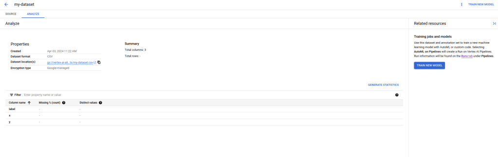
You now have several options to proceed. You can follow the link displayed on the right hand side to use Vertex AIs AutoML feature which will train a regression model on your data from scratch (be careful, there is an extra charge associated with that which goes far beyond the cost for the actual compute capacity needed, so do not do this if you just want to play). You can also analyze the data by clicking on the link “Generate statistics”.
Be patient, even for our tiny sample with 2000 items, this will take some time – when I tried this, it took about ten minutes. As a result, you will get the count of distinct values per column, and Vertex AI would also inform you about any missing values.
Let us now try to collect a bit more information on our dataset by using the Python API. The high-level API defines APIs which are specific for a given dataset type, but there is also an API that we can use to get information for an arbitrary dataset. Our repository contains an example that demonstrates how to use this in datasets/get_dataset.py. Let us run this.
python3 datasets/get_dataset.py
If you look at the output, you will find that it references a metadata schema that is in fact specific to the type of dataset that we have defined. The metadata schema is the URI of a file on GCS, and you can of course use gsutil to download a copy of this.
gsutil cp gs://google-cloud-aiplatform/schema/dataset/metadata/tabular_1.0.0.yaml .
more tabular_1.0.0.yaml
From this description, you will learn that a tabular dataset is really only a pointer to the data that is contains, which can either be stored in one or more files on GCS or in a BigQuery table. In addition to this, Google will only store some metadata like the creation time and a unique ID. Google will, however, add a metadata item to the metadata store that also references the dataset.
Text datasets
Let us now turn to a slightly more interesting type of datasets – text datasets. The basic workflow for text datasets is the same as for tabular datasets – we create the dataset (either via the SDK or on the console) and upload data. However, the format of the data is different – data is usually imported in JSON format that follows a specific schema which depends on the classification task. Let us use sentiment analysis as an example for which the schema is available here. Essentially, each item in our data (called a document) would be represented by a JSON object that looks as follows.
{
    "textContent" : "the actual text",
    "sentimentAnnotation": {
            "sentiment": 1,
            "sentimentMax": 2
    },
}
Here, the textContent is the actual data. The content of sentimentAnnotation – if present – contains the label, which consists of a score between 0 and maximal 10, and the sentimentMax value that specifies the maximum value (and should be the same for all documents in the set).
Instead of including the text content directly, the field textContent can also be replaced by a field textGcsUri which is the URI of a file stored on GCS, so that every record is represented by one file. Also note that only each line is valid JSON, while the full document is not – this is why the format is called JSON lines and has extension *.jsonl.
To try this, we again need a small sample dataset. As this is a series on Vertex AI, I could not resist the temptation to write a small script which asks Googles Gemini Pro model to do this for us. It uses few-shot learning to get a batch of ten records from the LLM, validates the content to see that it is valid, and repeats this until we have collected 100 valid documents which are then written to a file text.jsonl. You can either run this yourself
python3 datasets/generate_text_data.py
or use the file that I have included in the repository
cp datasets/text.jsonl .
In any case, we will again have to copy the file that you want to use to a GCS bucket as we did it before for the tabular dataset.
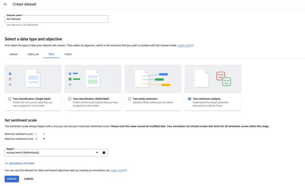
Once the upload is complete, you can create a dataset using the same workflow as for our tabular dataset, with the difference that you will have to select a text dataset with the objective sentiment analysis. Also note that you will have to specify the minimum and maximum sentiment score (0 and 2 in our case) and you will have to use a location that supports this feature which is not yet available in all locations. Let us call our dataset “text-dataset”.
Then proceed with the import as before by selecting the GCS location of the text.jsonl file that we have uploaded earlier. Again, the import takes some time. Note that the test data set that is included in the repository does actually contain duplicates, so when the import completes, you will only see 98 records, not 100 – this nicely demonstrates that Google does some work behind the scenes while you are waiting.
Let us now take a closer look at our dataset by running the script again that we have already used to display our tabular dataset, specifying the name and region of our new dataset – be sure to use the same region here as the one that you have selected when creating the dataset.
If you compare this to the output for our tabular dataset, you should see two interesting differences. First, this dataset has a different schema reflecting the fact that this is a text dataset, not a tabular dataset. Second the GCS bucket that is displayed is not the bucket that we have used for the upload, but a bucket that Google has generated for us. This reflects the fact that this time, the data itself is managed by Google and is more than just a reference.
It is instructive to actually visit the GCS bucket that Google has generated (which will be owned by you, so you can actually see it). You will find that behind the scenes, Google has created one blob for every item in the input. This allows the platform to also modify each item separately, and in fact, in the console window for this dataset, you can edit individual items and add, remove or change labels.
Corresponding to this, you can also export your dataset, either directly from the console or programmatically using the export_data method of the DatasetServiceClient. Here, exporting means that the data will be written to a GCS location of your choice from where you can further process it – I would not recommend to directly use the bucket controlled by Google for this purpose as this is supposed to be managed by Google exclusively.
This closes our short series on Vertex AI. Of course, there are many features that we have not yet touched upon, like notebook and the workbench, batch predictions, feature stores or the new platform components with GenAI specific services like the model garden, LLMs and vector storage. However, with the basic understanding that you will have gained if you have followed me up to this point, you should be well prepared to explore these features as well.
When we access a VertexAI predicition endpoint, we usually do this using the Google API endpoint, i.e. we access a public IP address. For some applications, it is helpful to be able to connect to a prediction endpoint via a private IP address from within a VPC. Today, we will see how this works and how the same approach allows you to also connect to an existing VPC from within a pipeline job.
VPC Peering
The capability of the Google cloud platform that we will have to leverage to establish a connection between VertexAI services and our own VPCs is called VPC peering, so let us discuss this first.
Usually, two different networks are fully isolated, even if they are part of the same project. Each network has its own IP range, and virtual machines running in one network cannot directly connect to virtual machines in another network. VPC peering is a technology that Google offers to bridge two VPCs by adding appropriate routes between the involved subnets.
To understand this, let us consider a simple example. Suppose you have two networks, say vpc-a and vpc-b, with subnets subnet-a (range 10.200.0.0/20) and subnet-b (10.210.0.0/20).
Google will then establish two routes in each of the networks. The first route called the default route sends all traffic to the gateway that connects the VPC with the internet. The second route called the subnet route (which exists for every subnet) has a higher priority and makes sure that traffic to a destination address within the IP address range of the respective subnet is delivered within the VPC.
As expected, there is not route that is connecting the two networks. This is changed if you decide to peer the two networks. Peering sets up additional routes in each of the networks so that traffic targeting a subnet in the respective peer network is routed into this network, thus establishing a communication channel between the two networks. If, in our example, you peer network-a and network-b, then a route will be set up for network-a that sends traffic with destination in the range 10.210.0.0/20 to network-b and vice versa. Effectively, we map subnet-b into the IP address space of network-a and subnet-a into the IP address space of network-b.
Note that peering is done on the network level and applies for all subnets of both networks involved. As a consequence, this can only work if the address ranges of the subnets in both networks do not overlap, as we would otherwise produce conflicting routes. This is the reason why peering does not work with networks created in auto-mode, but requires subnet mode custom.
Private prediction endpoints
Let us now see how VPC peering can be applied to access prediction endpoints from within your VPC using a private IP address. Obviously, we need a model to do this that we can deploy. So follow the steps in our previous post on models to upload a model to the Vertex AI registry (i.e. train a model, create an archive, upload the archive to GCS and the model to the registry) with ID vertexaimodel.
Next we will deploy the model. Recall that the process of deploying a model consists of two steps – creating and endpoint and deploying the model to this endpoint. When we want to deploy a model that can be reached from within a VPC, we will need to create what Google calls a private endpoint instead of an endpoint. This is very similar to an endpoint, with the difference that as an additional parameter, we need to pass the name of a VPC. Behind the scenes, Google will then create a peering between the network in which the endpoint is running and our VPC, very similar to what we have done manually in the previous section.
For this to work, we first need a few preparations. First, we need to set up our VPC, and we also create a few firewall rules that allow SSH access to machines running in this network (which we will need later), and allow ICPM and internal traffic.
Now we need to let Google know which IP address range it can use to establish a peering. This needs to be a range that we do not actively use. To inform Google about our choice, we create an address range with the special purpose VPC_PEERING. We also need to create a peering between our network and the service network that Google uses.
To create a private endpoint and deploy our model to it, we can use more or less the same Python code that we have used for an ordinary endpoint, except that we create an instance of the class PrivateEndpoint instead of Endpoint and pass the network to which we want to peer as additional argument (note, however, that private endpoints do currently not support traffic splitting, so the parameters referring to this are not allowed).
Let us try this – simply navigate to the directory networking in the repository for this series and execute the command
python3 deploy_pe.py --vpc=peered-network
Again this will probably take some time, but the first step (creating the endpoint) should only take a few seconds. Once the deployment completes, we should be able to run predictions from within our VPC. To be able to verify this, let us next bring up a virtual machine in our VPC, more precisely within a subnet inside our VPC that we need to create first. For that purpose, set the environment variable GOOGLE_ZONE to your preferred zone within the region GOOGLE_REGION and run
Next, we need to figure out under which network address our client can reach the newly created endpoint. So run gcloud ai endpoints list to find the ID of our endpoint and then use gcloud ai endpoints describe to print out some details. In the output, you will find a property called predictHttpUri. Take note of that address, which should be a combination of the endpoint ID, the domain aiplatform.googleapis.com and the ID of the model. Then SSH into our client machine and run a curl against that address (set URL in the command below to the address that you have just noted).
At first glance, this seems to be very similar to a public endpoint, but there are a few notable differences. First, you can use getent hosts in the client machine to convince yourself that the DNS name in the URL that we use does in fact resolve to a private IP address in the range that we have defined for the peering (when I tried this, I got 10.8.0.6, but the result could of course be different in your case). We can even repeat the curl command and use the IP address instead of the DNS name, and we should get the same result.
The second thing that is interesting here is we did not have to associate our virtual machine with any service account. In fact, everyone who has access to your VPC can invoke the endpoint, and there is no additional permission check. This is in contrast to a public endpoint which can only be reached when passing a bearer token in the request. So you might want to be very thoughtful about who has access to your network before deploying a model to a private endpoint – this is in fact not private at all.
We also remark that creating a private endpoint is not the only way to reach a prediction endpoint via a private IP address. The alternative approach that Google offers you is called private service connect which provides a Google API endpoint at an IP address in your VPC. You can then deploy a model as usual to an ordinary endpoint, but use this private access point to run predictions.
Connecting to your VPC from a VertexAI pipeline
So far, we have seen how we can reach a prediction endpoint from within our VPC using a peering between the Google service network and our VPC. However, this also works in the other direction – once we have the peering in place, we can also reach a service running in our VPC from within jobs and pipelines running on the VertexAI platform.
Let us quickly discuss how this works for a pipeline. Again, the preconditions that you need are as above – a VPC, a reserved IP address range in that VPC and a peering between your VPC and the Google service network.
Once you have that, you can build a pipeline that somehow accesses your VPC, for instance by submitting a HTTP GET request to a server running in your VPC. When you submit this job, you need to specify the additional parameter network as we have done it when creating our private endpoint. In Python, this would look as follows.
#
# Make sure that project_number is the number (not the ID) of the project
# you are using
#
project_number = ...
#
# Create a job
#
job = aip.PipelineJob(
    display_name = "Connectivity test pipeline",
    template_path = "connect.yaml",
    pipeline_root = pipeline_root,
    location = location,
)

#
#
# Submit the job
job.submit(service_account = service_account,
           networkm= f"projects/{project_number}/global/networks/{args.vpc}")
Again, this will make Vertex AI use the peering to connect the running job to your network so that you can access the server. I encourage you to try this out, just modify any of the pipelines we have discussed in our corresponding post to submit a HTTP request to a simple Flask server or an NGINX instance running in your VPC to convince yourself that this really works.
This closes our post for today. Next time, we will take a look at how you can use Vertex AI managed datasets to organize your training data.
When you assemble and run a custom job, the Vertex AI platform is not aware of the inputs that you consume and the outputs that you create in this job, and consequently, it is up to you to create execution and artifact metadata and the corresponding relations between executions, input artifacts and output artifacts. For pipelines, the situation is different, as you explicitly declare input and output artifact of each component that is executed as part of a pipeline. Thus you could expect that the platform takes over the task to reflect this in the metadata, and in fact it does. Today, we take a closer look at the metadata that a pipeline run produces.
Pipeline jobs, executions and artifacts
As a starting point for what follows, let us first conduct a little experiment. Starting from the root directory of the cloned repository run the following commands to clean up existing metadata (be careful, this will really delete all metadata in your Vertex AI project) and submit a pipeline.
cd pipelines
python3 ../metadata/list_metadata.py --delete
python3 submit_pipeline.py
Then wait a few minutes until the pipeline run is complete and display the metadata that this pipeline run has created.
python3 ../metadata/list_metadata.py --verbose
We can see that Vertex AI will create a couple of metadata objects automatically. First, we see artifacts representing the input and outputs of our components, like the model, the test and validation data and the metrics that we log. Then we see one execution of type system.ContainerExecution for each component that is being executed, and the artifacts are correctly linked to these executions.
There is also an execution of type system.Run that apparently represents the pipeline run. Its metadata contains information like the project and the pipeline run ID, but also the parameters that we have used when submitting the pipeline.
Finally, Vertex AI will create two nested contexts for us. The first context is of type system.PipelineRun and represents the run. All executions and artifacts for this run are living inside this context. In addition, there is a context which represents the pipeline (type system.Pipeline) and the pipeline run is a child of this context. When we submit another run of the pipeline, then a new run context will be created and will become a child of this pipeline context as well. Here is a diagram summarizing the structure that we can see so far.
Experiment runs and pipelines
Let us now see how this changes if we specify an experiment when submitting our pipeline (the submit method of the PipelineJob has a corresponding parameter). In this case, the SDK will locate the pipeline run context and associate it with the experiment, i.e. it will add it as child to the metadata context that represents the experiment. Thus our pipeline run context has two parent contexts – the context representing the experiment and the context representing the pipeline. Let us try this.
This should give an output reflecting the following diagram.
If you now open the Vertex AI console and navigate to the “Experiments” tab, you will see our newly created experiment and inside this experiment, there is a new run (the name of this run is a combination of the pipeline name and a timestamp). You can also see that the metadata that is attached to the pipeline execution, in particular the input parameters, show up as parameters, and that all metrics that we log using log_metric on an artifact of type Metric will automatically be displayed in the corresponding tab for the pipeline run. So similar to what we have seen for custom jobs, you again have a central place from which you can access parameters, metrics and even the artifacts created during this pipeline run. However, this time our code inside the pipeline components does not have to use any reference to the Google cloud framework, we only interact with the KFP SDK, which makes local execution and unit testing a lot easier.
Using tensorboards with Vertex AI pipelines
We have seen that logging individual metrics from within a pipeline is very easy – just add an artifact of type Metrics to your component and call log_metrics on that, and Vertex AI will make sure that the data appears on the console. However, for time series, this is more complicated, as Vertex AI pipeline are apparently not yet fully integrated with the Vertex AI tensorboards.
What options do we have if we want to log time series data from within a component? One approach could be to simply use start_run(..., resume = True) to attach to the pipeline run and then log time series data as we have done it from within a custom job. Unfortunately, that does not work, as start_run assumes that the run you are referring to is of type system.ExperimentRun but our run is of type system.PipelineRun.
You could of course create a new experiment run and use that experiment run to log time series data. This works, but has the disadvantage that now every run of the pipeline will create two experiment runs on the console, which is at least confusing. Let us therefore briefly discuss how to use the tensorboard API directly to log data.
The tensorboard API is built around three main classes – a Tensorboard , a TensorboardExperiment and a TensorboardRun. A Tensorboard is simply that – an instance of a managed tensorboard on Vertex AI. Usually there is no need to create a tensorboard instance manually, as Vertex AI will make sure that there is a backing tensorboard if you create an experiment in the init function (the default is to use the same tensorboard as backing tensorboard for all of your experiments). You can access this tensorboard via the backing_tensorboard_resource_name attribute of an Experiment.
Once you have access to the tensorboard instance, the next step is to create a tensorboard experiment. I am not sure how exactly Google has implemented this behind the scenes, but I tend to think of a tensorboard experiment as a logging directory in which all event files will be stored. If you make sure that the name of a tensorboard experiment matches the name of an existing Vertex AI experiment, then a link to the tensorboard will be displayed next to the experiment in the Vertex AI console. In addition, I found that there is a special label vertex_tensorboard_experiment_source that you will have to add with value vertex_experiment to avoid that the tensorboard experiment is displayed as a separate line in the list of experiments.
Next, you will need to create a tensorboard run. This is very similar to an experiment run and – at least in a local tensorboard installation – corresponds to a directory in the logging dir where event files are stored.
If you actually want to log time series data, you will do so by passing a label, for instance “loss”, a value and a step. Label and value are passed as a dictionary, the step is an integer, so that a call looks like this.
#
# Create a tensorboard run
#
tb_run = ...
#
# Log time series data to it
#
tb_run.write_tensorboard_scalar_data({
                            "loss" : 0.05
                        }, step = step)
All values with the same label – in our case “loss” – form a time series. However, before you can log data to a time series in this way, you will actually have to create a time series within the tensorboard run. This is a bit more complicated than it sounds as creating a time series that already exists will fail, so you need to check upfront whether the time series exists. To reduce the number of API calls needed, you might want to keep track of which time series have already been created locally.
In order to simplify the entire process and in order to allow for easier testing, I have put all of this into a utility class defined here. This class can be initialized once with the name of the experiment you want to use, a run name and your project ID and location and then creates the required hierarchy of objects behind the scenes. Note, however, that logging to a tensorboard is slow (I assume that the event file is stored on GCS so that appending a record is an expensive operation), so be careful not to log too many data points. In addition, even though our approach works well and gives you a convenient link to your time series in the Vertex AI console, the data you are logging in this way is not visible in the embedded view which is part of the Vertex AI console, but only in the actual tensorboard instance – I have not yet figured out how to make the data appear in the integrated view as well.
The standard pipeline that we use for our tests already uses tensorboard logging in this way if you submit it with an experiment name as above. Here is how the tensorboard instance will look like once the training step (which logs the training loss) is complete.
Some closing remarks
Pipeline metadata is a valuable tool, but does not mean that you do not have to implement additional mechanisms to allow for full traceability. If, for instance, you train a model on a dataset that you download from some location in your pipeline and then package and upload a new model version, the pipeline metadata will help you to reconstruct the pipeline run, but the entry in the model registry has no obvious link to the pipeline run (unless maybe the URI which will typically be some location inside the pipeline root), you will still need to track the version of your Python code for defining the model and the training script separately, and you can also not rely on the pipeline metadata alone to document the version of data you use that originates from outside of Vertex AI.
I tend to think of pipeline metadata as a tool which is great for training – you can conduct experiment runs, attach metrics and evaluation results to runs, compare results across runs and so forth – but as soon as you deploy to production, you will need additional documentation.
You might for instance want to create a model card that you add to your model archive. This model card can be assembled as a markdown or HTML artifact inside your pipeline declared as component output via Output[Markdown](VertexAI will even display the model card artifact for you).
Of course this is just a toy example, and in general you might want to use a toolkit like the Google Model Card Toolkit to assemble your model card, typically using metadata and metrics that you have collected during your pipeline run. You can then distribute the model card to a larger group without depending on access to Vertex AI metadata and archive it, maybe even in your version control system.
Vertex AI metadata is also comparatively expensive. At the time of writing, Google charges 10 USD per GB and month. Even standard storage at european locations is around 2 cents per GB and month, and archive storage is even less expensive. So from time to time, you want to clean up your metadata store and archive the data. As an example of how this could work, I have provided a script cleanup.py in the pipelines directory of my repository. This script removes all metadata (including experiments) as well as pipeline runs and custom job executions older than a certain number of days. In addition, you can chose to archive the artifact lineage into a file. Here is an example which will remove all data older than 5 days and write the lineage information into archive.dat.
This closes our blog post for today. In the next post, we will turn our attention away from pipelines to networking and learn how you can connect jobs running on Vertex AI to your own VPCs and vice versa.
In our previous post, we have covered the process of creating pipeline components, defining a pipeline and running the pipeline in Vertex AI. However, parts of this appeared to be a bit mysterious. Today, we will take a closer look at what is going on behind the scenes when we create and run a pipeline
Deep dive into component creation
To be able to easily and interactively inspect the various types of Python objects involved, an interactive Python shell is useful. You might want to use ipython3 for that purpose or you might want to run the following commands to install a kernel into our environment and add the kernel to the Jupyter configuration so that you can run all this in a Jupyter notebook.
As a starting point for our discussion, it is helpful to recall what a Python decorator is doing. Essentially, a decorator is a device to wrap a function into a different function or – more precisely – a callable which can either be a function or a Python object with a __call__ method. Therefore, a decorator is a function which accepts a function as input and returns a callable. This callable will then be registered under the name of the original function in the namespace, so effectively replacing the decorated function by the new callable.
Let us take a closer look at this for the example of a pipeline component. Suppose we have a very simply pipeline component.
from kfp import dsl
from kfp.dsl import Output, Artifact, Dataset

@dsl.component(base_image = "python:3.9")
def my_component(msg : str, data : Output[Dataset]):
    print(f"Message: {msg}")
When the Python interpreter hits upon this piece of code, it will call the decorator – i.e. the function kfp.dsl.component_decorator.component– with the first argument being your my_component function (and the remaining parameters being the parameters of the decorators like base_image in our case). This decorator function uses inspection to analyze the parameters of your function and then returns an instance of kfp.dsl.python_component.PythonComponent which then becomes known under the name my_component . Let us verify this in our interactive Python session and learn a bit about our newly created object.
type(my_component)
my_component.__dict__.keys()
We see that our new object has an attribute python_func. This is in fact the wrapped function which you can inspect and run.
import inspect
inspect.getsource(my_component.python_func)
my_component.python_func("Hello", data = None)
Another interesting attribute of our object is the component_spec. This contains the full specification of the container that will implement this component (you might want to take a look at this, but we will get back to it later) including image, command, arguments and environment, and the description of inputs and outputs of our component.
Assembling a pipeline
We now have a component. As a next step, we will assemble our components into a pipeline. As we have seen, this usually happens with a piece of code like this.
So here we call our component – but in fact, as our component has been replaced by the PythonComponent, we do actually not call our component but end up in the __call__ method of PythonComponent. This method will create a representation of the component at runtime, i.e. an instance of a PipelineTask. In addition to a component specification, this object now also contains the inputs and outputs of our component (we see actual values, not just descriptions – note that artifacts are represented by placeholders).
But how do the components actually end up in a pipeline? Why is there no need to explicitly call something along the lines of my_pipeline.add(my_component)? This is where the magic of decorators and the magic of context managers join forces…
To understand this, let us go back a step and think about what happens when the Python interpreter hits upon the line @dsl.pipeline. At this point, the pipeline decorator function defined here is invoked and receives our function my_pipeline as argument. After some intermediate calls, we end up constructing a GraphComponent which is the object actually representing a pipeline. In the constructor of this component, we find the following code snippet.
with pipeline_context.Pipeline(
                self.component_spec.name) as dsl_pipeline:
    pipeline_outputs = pipeline_func(*args_list)
So we eventually run the code inside the function body of our my_pipeline function where, as we already know, we create a PipelineTask for every component. But we do this within a pipeline context, i.e. an instance of the class Pipeline which implements the Python context manager interface. So the __enter__ method is called, and this method sets the variable pipeline_task.PipelineTask._register_task_handler.
Now the point is that the function pointed to by this variable is invoked in the constructor of a PipelineTask (this happens here)! Thus for every component created inside a function that carries the pipeline decorator, a call into the pipeline context, more precisely into the add_task method of the pipeline context, will be made automatically, meaning that all components that we create here will automatically be registered with the pipeline. Its not magic, just some very clever Python code…
for connecting inputs and outputs works. When this is executed, _train is an instance of a PipelineTask which does actually have an attribute called outputs, and we have seen that this is a dictionary with one entry for each output that we declare. This explains why we can get the outputs from this dictionary and pass them another component as input.
An important lesson from all this is that the code in the pipeline definition gets executed at build time, but the code in the component definition is actually never executed unless we submit the pipeline. This implies that trivial errors in the code are detected only if you really submit the pipeline (and this takes some time, as every step provisions a new container on the Google platform). Therefore it is vitally important to test your code locally before you submit it, we will see a bit later in this post how this can be done.
Pipeline execution
We have seen above that the component specification that is part of a Python component or a pipeline task does already contain the command (i.e. the entrypoint) and the arguments which will be used to launch the container. Structurally (and much simplified, if you want to see the full code take a look at the generated pipeline IR YAML file after compilation), this command in combination with the arguments looks as follows.
#
# First install KFP inside the container
#
python3 -m pip install kfp
#
# Create a Python module holding the code
# of the component
#
printf "%s" <<code of your component>> > "ephemeral_component.py"
#
# Run KFP executor pointing to your component
#
_KFP_RUNTIME=true python3 -m kfp.dsl.executor_main \
  --component_module_path  "ephemeral_component.py" \
  --executor_input <<executor input>> \
  --function_to_execute <<your component code>>
Let us go through this step by step. First, we invoke pip to make sure that the KFP package is installed in the container (in the full version of the code, we can also see that apt-get is used to install pip if needed, which makes me think about what happens if we use a base image that is not based on a Debian distribution – I do not think that this implicit requirement is mentioned anywhere in the documentation). We then store the code of the pipeline component in a file called ephemeral_component.py, and run the KFP executor main entry point.
After loading your code as a module, this will create an instance of an executor and invoke its execute method. This executor is created with two arguments – the function to be executed (corresponding to the last argument in the command line sketched above) and the executor input (corresponding to the second to last line in the command above).
The executor input is a JSON structure that contains the information that the executor needs to construct input and output artifacts. Here is an example.
In this example, the input only consists of parameters, but in general, the input section can also contain artifacts and would then look similarly to the output section.
In the output section, we can find a description of each artifact created by our component. This description contains all the fields (name, metadata, schema and URI) that are needed to instantiate a Python representation of the artifact, i.e. an instance of the Artifact class. In fact, this is what the executor does – it uses the data in the executor input to instantiate parameters and input and output artifacts and then simply calls the code of the component with that data. Inside the component, we can then access the artifacts and parameters as usual.
Note that the output section also contains an execution output file. This is a file to which the executor will log outputs. When you run a pipeline on Vertex AI, this executor output is stored in your GCS pipeline root directory along with the real artifacts. If your component returns any parameter values (a feature which we have mentioned but not yet discussed so far), the executor will add the output parameter values to this file as well so that the engine can get it from there if needed.
We can now understand what execution of a pipeline really means. The engine executing your pipeline needs to inspect the DAG derived from the pipeline to understand in what order the components needs to run. For each component, it then assembles the executor input and runs the container defined in the component specification with the command and arguments as sketched above. It then looks at the execution output written by the file and extracts the outputs of the components from there to be able to pass it as input to other components if needed.
There is one little step that we have not discussed so far. We have learned that an artifact has an URI (pointing to GCS) and a path (pointing into a local file system inside the container). How is the URI mapped to the path and why can the component code access the artifact?
Again, the source gives us a clue, this time the code of the Artifact class itself in which we see that the path attribute is decorated as a Python property, turning it into what the Python documentation calls a managed attribute. If you look at the underlying function, you will see that this simply translates the URI into a local path by replacing the “gs://” piece of the GCS location with “/gcs” (or whatever is stored in _GCS_LOCAL_MOUNT_PREFIX). The executing engine needs to make sure that this directory exists and contains a copy of the artifact, and that changes to that copy are – at least for output artifacts – replicated back to the actual object on GCS. Vertex AI does this by mounting the entire bucket using gcsfuse, but the KFP internal executor seems to simply create a copy at least if I read this code correctly)
Testing pipelines locally
Having a better understanding of what happens when a component is executed now puts in a position to think about how we can execute a component locally for testing purposes.
First, let us discuss unit testing. If we have a function annotated as a component, we have learned that calling this function as part of a unit test is pointless as the code of the component will not even be run. However, we can of course still access the original function as my_component.python_func and call it as part of a unit test (or, more conveniently, we can use the execute method of a Python component that does exactly this). So in order to run a unit test for a component define like this
we could come up with a Python unit test like this (designed to work with pytest).
from unittest.mock import Mock
import os

def test_create_data(tmp_path):
    output_dir = f"{tmp_path}/outputs/"
    os.mkdir(output_dir)
    #
    # Make sure that environment variables are set
    #
    os.environ["GOOGLE_PROJECT_ID"] = "my-project"
    os.environ["GOOGLE_REGION"] = "my-region"
    #
    # Import the file where all the components are defined
    #
    import pipeline_definition
    #
    # Prepare mocked artifacts
    #
    training_data = Mock(
        uri = "gs://test/training_data",
        path = f"{output_dir}/training_data"
    )
    validation_data = Mock(
        uri = "gs://test/training_data",
        path = f"{output_dir}/validation_data"
    )
    pipeline_definition.create_data.execute(size = 10,
                            training_data = training_data,
                            validation_data = validation_data)
    #
    # Do whatever validations have to be done
    #
So we first import the file containing the component definitions (note that environment variables that we refer to need to be defined before we do the import as they are evaluated when the import is processed) and then use execute to access the underlying function. Output artifacts are mocked using a local path inside a temporary directory provided by pytest. Inside the test function, we can then access the outputs and run whatever validations we want to run.
If your code invokes Google API calls, do also not forget to mock those (maybe you even want to patch the entire module to be on the safe side) – you do not want to be caught be surprise by a high monthly bill because you accidentally spin up endpoints in your unit tests that you run several times a day as part of a CI/CD pipeline…
After unit testing, there is typically some sort of integration test. A possible approach to doing this without having to actually submit your pipeline is to use the magic of the KFP executor that we have seen above to your advantage by invoking the executor with your own executor input in order to run containers locally. Roughly speaking, here is what you have to do to make this work.
First, we need to look at the component specification and extract input and output parameters and artifacts which will be instances of either InputSpec or OutputSpec. For each input and output, we have determine whether it represents a parameter or an artifact based on the value of the type field. For a parameter, we determine the value that the parameter should have. For artifacts, we need to assemble a URI.
For each input and output, we can then add a corresponding snippet to the executor input. We then pass this executor input and a command assembled according to the logic shown above into a docker cointainer in which we run our image. To be able to preserve artifacts across component runs so that we can test an entire pipeline, we will also want to mount a local filesystem as “/gcs” into the container.
Alternatively, we can also run our component outside of a container by using the KFP executor. When we do this, however, we need to apply an additional trick as by default, this will use a local path starting with “/gcs” which is usually not accessible by an ordinary user. However, we have seen that this prefix is a variable that we can patch to point into a local file system of our choice before running the executor.
I have put together a script showing how to do all this in my repository. To try this out, switch into the pipeline subdirectory of the cloned repository and run
#
# Preload the Python images that we use
#
docker pull python:3.9
docker pull $GOOGLE_REGION-docker.pkg.dev/$GOOGLE_PROJECT_ID/vertex-ai-docker-repo/pipeline:latest
#
# Run the actual script
#
python3 run_locally.py --no_container
which will run our pipeline without using containers. If you drop the parameter, the component will execute inside a container and you will see some additional output that the executor generates, including the full executor input that we assemble. This simple script still has a few limitations, it is for instance not able to handle artifacts which are a list or a dictionary, but should work fine for our purposes.
One closing remark: looking at the documentation and the source code, it appears that newer versions of KPF like 2.6 come with a functionality to run components or even pipelines locally. As at the time of writing , the Google SDK has a dependency on KFP 2.4 which does not yet offer this functionality, I have not tried this, but I expect it to work somehow in a similar fashion.
We now have built a solid understand of what is going on when we assemble and run a pipeline. In the next post, we will take a closer look at how Vertex AI reflects pipeline runs in its metadata and how we can log metrics and parameters inside a pipeline.
So far, we have worked with individual jobs. However, a typical machine learning flow is more complicated than this – you might have to import data, transform it, run a training, validate the outcomes or do a hyperparameter search, package a model and deploy it. Instead of putting all this into a single job, VertexAI allows you to define pipelines that model this sort of flow.
Before we start to discuss pipelines, let us describe the problem that they are trying to solve. Suppose you have a standard machine learning workflow consisting of preparing your input data, training a model, performing a validation and finally packaging or even deploying your model. During each of these steps, there are some artifacts that you create – a training data set, validation metrics, or a trained and packaged model.
Of course you could put all of this into a single custom job. However, if that job fails, all artifacts are lost until you implement some sort of caching yourself. In addition, monitoring this job to understand where you are in the process also requires a custom implementation, and we have seen in the previous posts that while you can manage experiment runs and metadata in a custom job, this requires a bit of effort.
Pipelines are a different way to address this problem. Instead of modelling a workflow and dependencies explicitly in your code, you declare individual components, each of which has certain inputs and outputs, and declare a pipeline that contains these components. In the background, VertexAI will then build a dependency graph, run your components, trace and cache inputs and outputs and monitor the execution.
VertexAI pipelines are based on Kubeflow which, among other things, implements a DSL (domain specific language) to describe components and jobs and Python decorators that allow you to model all this in Python code. If you work with pipelines, you will first declare your components, assemble these components into pipelines, create a pipeline specification and finally submit this to the platform for execution.
Let us now go through all of these steps before diving deeper into some topics in upcoming posts.
Component creation
Even though Kubeflow offers several types of components, most components that we will use will be what is called a lightweight Python component. Essentially, this is simply an ordinary Python function annotated as a component, like this.
from kfp import dsl

@dsl.component(
    base_image = "python:3.9")
def do_something():
    # some Python code
When the pipeline is executed, each component will be run as a separate container. We will look in detail at the process of executing a pipeline component a bit later, but essentially the execution engine will spin up the container specified by the base_image parameter of the annotation and run the code within the function inside this container.
This is simple, but has an important implication – the code within the function needs to be fully standalone. As a consequence, no global variables can be referenced, imports have to be done within the body of the function and, most importantly, we cannot invoke any function or class which is not defined inline inside the component function. If, for instance, we want to instantiate a PyTorch model we either have to pull the corresponding class definition into the function or we have to place the file with the model code in the container.
To be useful, a component typically needs to process inputs and produce outputs. Let us see how this works for pipeline components. In VertexAI (and KFP) pipelines, there are two different types of inputs our outputs that your function can declare – parameters and artifacts
A parameter is just an input to your function (i.e. a Python parameter) that is either defined at compile time when assembling the components into a pipeline or – more useful – when you actually submit the pipeline for execution (there are also output parameters, we get back to this). Behind the scenes, the execution engine serializes the value of a parameter into a JSON structure and (by some magic that we will look at in more detail in one of the upcoming posts) calls your component function passing this value as an ordinary Python parameter. KFP supports strings, integers, floats, boolean values and dictionaries and lists as parameters.
While parameters are passed by value, there is a second type of input a function can take and which I tend to think of as passing arguments by reference. This is mostly applied to large pieces of data like models or datasets that you do not want to pass around as a JSON object but as what is called an artifact. Inside the Python code, an artifact is represented by a Python object that has – in addition to its name – three major attributes. First, every artifact has a URI which is the name of a blob on GCS (KFP itself also supports other storage solutions like S3 and Minio). The idea is that within your Python code, the artifact represents the actual artifact stored under this URI. Second, there is a path which also points to the actual artifact but on local storage (we will explain this in a minute), and third there is a metadata property which is just a dictionary which you can use to attach metadata to an artifact.
Let us look at an example to see how this works in practice. Consider the following code snippet that defines a component called train.
from kfp import dsl
from kfp.dsl import Output, Model, Dataset, Metrics


@dsl.component(
    base_image = ...,
)
def train(epochs : int,
          lr : float,
          data : Input[Dataset],
          trained_model : Output[Model],
          metrics: Output[Metrics]):
    # Train
    ...

    # Log some metrics
    metrics.log_metric("final_loss", loss.item())
    #
    # Store trained model as state dir
    #
    torch.save(_model.state_dict(), trained_model.path)
First, we see that all Python function parameters are annotated – this is required for pipeline components, as the runtime needs the type information to do its job. In our example, epochs and lr are parameters. Their values will be injected at runtime, and in the body of your function, you can access them as usual.
The other inputs – data, trained_model and metrics – are artifacts of type dataset, model and metrics (there is also a type for generic artifacts). The annotations of these artifacts do not only specify the type, but also whether this is input or output. In your Python code, you can access attributes like metadata directly to read or modify metadata (though you should only do this for output artifacts). You can also call functions like log_metric on a metrics artifact to log the actual metrics which will later be displayed on the VertexAI console. In fact, Output is a Python type annotation (see PEP 593) so that the parameter model can be treated as being of type Model inside the code.
To access the content of the actual artifact, for instance our model, you use the path property of the artifact. This is a string containing a path to the actual object on the local filesystem. When you run your pipeline, VertexAI will mount the GCS bucket where your objects are located (the so-called pipeline root) via gcsfuse into the local container file system and sets up the value of path for you accordingly. You can now read from this and write to it as needed, for instance to store model weights as in the example above. Via the file system mount, the changes will then be written back to the underlying GCS bucket. So while the actual data comprising the artifact is living on GCS it can be accessed via the Python artifact object – the trained_model in our case – this is why I tend to think of this as a reference.
Pipeline creation
We have now seen you individual components can be created by using decorators (these components are called Python components, there are also more general components called container components but we will not discuss those today). Next we will have to patch these components together into a pipeline. Not surprisingly, this is again done using decorators, and again not surprisingly, the decorator we use is called pipeline . Here is an example.
@dsl.pipeline(
    name = "my-pipeline"
)
def my_pipeline(epochs : int, lr : float, training_items : int):
    _create_data = create_data(training_items = training_items)
    train(google_project_id = google_project_id,
                  google_region = google_region,
                  epochs = epochs,
                  lr = lr,
                  data = _create_data.outputs['data'])
This code snippet defines a pipeline with two steps, i.e. two components, called create_data and train . At the top, we again have an annotation that specifies the name of the pipeline. Within the body of the function carrying this annotation, we then simply call our pipeline components to add them to the pipeline. However, this call does not actually run the code defined for the invidual components but is diverted (thanks to the @component annotation) to a method of the KFP framework which adds the component definition to the pipeline. This looks a bit like black magic – we will take a deeper look at how exactly this works in the next post. So bear with me and simply accept this magic for the time being.
We also see how parameters and artifacts are handled. In our case, the pipeline itself has three parameters that we will define when we actually submit the pipeline. Again these parameters are annotated so that the framework can derive their type and deal with them.
In our example, we also use the output of the first step as input for the second step. To do this, we capture the output of the first step (again, this is not really the output of the annotated function but the output of the wrapper in which the framework wraps our original function) which is a Python object which has – among others – a property called outputs . This is a dictionary with keys being the names of the output parameters of our step, and we can use these keys to feed the data as input artifacts into the next step.
By chaining steps in this way, we also inform VertexAI about the dependencies of our components. In our example, the second step can only start once the first step is complete, as it uses the output of the second step, so there is a dependency. Behind the scenes, this information will be assembled into a directed acyclic graph (DAG) in which the vertices are the components and edges represent dependencies. When running our pipeline, components that can run in parallel because there are no dependencies will also be scheduled to run in parallel, but where needed the execution is serialized.
The output of the component invocation that we capture in the variable _create_data (the underscore is really just an arbitrary naming convention that I use, any name will do) is also useful for a second purpose – specifying the execution environment. For that purpose, this output (which is actually of type PipelineTask) has a set of methods like set_cpu_limit or set_memory_request to define limits and requests for the later execution (designed to run on a Kubernetes platform with the usual meaning of requests and limits, but this is not guaranteed by the framework). In particular, you can use set_accelerator_type to request a GPU of a specific type. Here is an example.
When playing with this, I experienced a strange problem – if I did not request at most four CPUs for a machine using a T4 GPU, the output of my Python script did not show up in the logs. There is even a ticket for this recommending to define a higher CPU limit (as I have done it above) as a workaround, so until this is resolved you will probably have to live with that and the additional cost.
Compiling a pipeline
We now have our beautiful pipeline in Python. This is nice, but to submit a pipeline we actually need to convert this into something that the VertexAI engine can process – a pipeline definition in what is called IR YAML (intermediate representation YAML). This contains among other data the specification of the individual components of the pipeline, information on how to execute them (we will get deeper into this when we talk about the details of component execution in one of the next posts) and the DAG that we have constructed.
To translate the Python representation into an IR YAML file, we use a component called the compiler. In the most common case, this only requires two parameters – the pipeline that we want to compile and the name of a file to which we write the YAML output.
Depending on the file name extension, the compiler will either create JSON or (recommended by the documentation) YAML output. We will take a closer look at the generated output in the next post in this series. We also note that it is possible to compile individual components and to load components from YAML files, so you could build a library of reusable components in YAML format as well.
Submitting a pipeline
Let us now submit the pipeline. It is important to understand that the YAML file that we have just created is all that actually gets uploaded to the VertexAI platform and contains all information that we need to run the pipeline, our Python code is just a local artifact (but shows up again in different form in the YAML file). To submit a pipeline to run as what is called a pipeline job, we first create a pipeline job object from the compiled YAML and then submit it.
Here, the template_path argument specifies the path to the compiled YAML file. The pipeline root parameter specificies a directory path in a GCS bucket under which all artifacts created during this pipeline run will be stored. You can also specify the values of parameters at runtime here (in fact, you will have to do this for all parameters which are not fixed at build time). In addition, you create a job in a specific project and region as usual.
Note the service account parameter which has a meaning similar to a custom job and is the service account under which all steps of this pipeline will execute.
Let us now try this with a real example. In my repository (that you should have cloned by now if you have followed the instructions in the introduction to this series), I have prepared a sample pipeline that uses all of this. To run this pipeline execute the following commands, starting from the root of the repository.
cd pipelines
# Will create the IR yaml
python3 pipeline_definition.py
# will submit the pipeline
python3 submit_pipeline.py
Once the pipeline is submitted, it is instructive to take a look at the graphical representation of the pipeline in the VertexAI console in the pipeline tab. Your newly submitted pipeline should show up here, and as you click on it, you should see a screen similar to the following screenshot.
What we see here is a graphical representation of the DAG. We see, for instance, that the validation step depends – via the trained model – on the training step, but also on the data creation.
On this screen, you can also click on one of the artifacts or steps to see more information on it in an additional panel on the right. For a step, you can navigate to the job itself (VertexAI will in fact create one custom job for each step) and its logs. For an artifact, you can click on “View lineage” to jump to the metadata screen where you will find that VertexAI has created metadata entries for our metrics, models and datasets but also for the steps and has associated artifacts to execution as we have done it manually when working with custom jobs.
When you submit the exact same pipeline again, you will produce a second pipeline run but this run will complete within seconds. This is the power of caching – VertexAI realizes that neither the jobs nor the input has changed and therefore skips all steps that would produce the same output again. This is very useful if you modify one of the later steps in the pipeline or if a step fails as it avoids having to re-run the entire pipeline again.
This concludes our short introduction. In the next post, we will shed some light on the apparent magic behind all this and learn how exactly components and pipelines are built and executed.
One of the core functionalities of every machine learning platform is traceability – we want to be able to track artifacts like models, training jobs and input data and tie all this together so that given a model version, we can go back all the way to the training data that we have used to train that version of the model. On VertexAI, this is handled via metadata which we will discuss today.
Metadata items and their relations
Let us start with a short introduction into the data model behind metadata. First, all metadata is kept ´behind the scenes in a metadata store. However, this is not simply a set of key-value pairs. Instead, the actual metadata is attached to three types of entities that populate the metadata store – artifacts, executions and contexts. Each of these entities has a resource name, following the usual naming conventions (with the metadata store as the parent), and a metadata field which holds the actual metadata that you want to store. In addition, each item has a display name and refers to a schema – we will come back to this later – plus a few fields specific for the respective entity.
Why these three types of metadata? The idea is that artifacts are the primary objects of interest. An artifact can be used as an input for a training run, like a dataset, or can be an output, like a model. Executions are the processes that consume and produce artifacts. Finally, there might be a need to group several executions together because they are somehow related, and this is the purpose of a context (at first glance, this seems to be based on MLMetadata which is part of TFX).
To model these ideas, the different types of metadata entities have relations that can be set and queried via API calls – they form a graph, called the lineage graph. For instance, an execution has a method assign_input_artifact to build a relation between an artifact and an execution, and a method get_input_artifact to query for these artifacts. Other types of entities have different relations – we can add an execution to a context and we can also build context hierarchies as a context can have children. Here is a graphical overview of the various relations that our metadata entities have.
Schemata, experiments and experiment runs
So far, this has been an abstract discussion. To make this concrete, we need to map this general pattern to the objects we are usually working with. An artifact, for instance, could be a model or a dataset – how do we distinguish between these types?
Instead of introducing dedicated objects for these different types of artifacts, VertexAI uses schemas. A schema describes the layout of the metadata but also serves to identify what type of entity we are looking at. Here is an API request that you can submit to get a list of all supported schemas.
Not every schema makes sense for every type of metadata entity. In the output of the statement above, you will find a schemaType field for each of the schemas. This fields tells us whether the respective schema describes an artifact, an execution or a context.
In the SDK code, the used schemas per type are encoded in the modules in aiplatform.metadata.schema.system . There is, for instance, a module artifact_schema.py which contains all schemas that can be used for artifacts (there are some schemas, however, in the output of the REST API that we call above which do not appear in the sourcecode). lf we go through these modules and map artifact types to schemas, we get the following picture.
Let us quickly discuss the most important types of schemas. First, for the schema type Artifact, we see some familiar terms – there is the generic artifact type, there are models, datasets and metrics.
Let us now turn to executions. As already explained, an execution is representing an actual job run. We see a custom job execution as well as a “Run” (which seems to be a legacy type from an earlier version of the platform) and a “ContainerExecution”. For the context, we see four different options. Today, we will talk about experiments and experiment runs and leave pipelines and pipeline runs to a later post.
An experiment is supposed to be a group of executions that somehow belong together. Suppose, for instance, you want to try out different model architectures. For that purpose, you build a job to train the model and a second job to evaluate the outcomes. Then each architecture that you test would correspond to an experiment run. For each run, you execute the two jobs so that each run consists of two executions. Ideally, you want to be able to compare results and parameters for the different runs (if you have ever taken a look at MLFlow, this will sound familiar).
This fits nicely into our general pattern. We can treat our trained model as artifact and associate this with the execution representing the training job. We can then associate the executions with the experiment run which is modelled as a context. The experiment is a context as well which is the parent of the experiment run, and everything is tied together by the relations between the different entities sketched above.
Creating metadata entities
Time to try this out. Let us see how we can use the Python SDK to create metadata entities in our metadata store. We start with artifacts. An artifact is represented by an instance of the class aiplatform.metadata.artifact.Artifact. This class has a create method that we can simply invoke to instantiate an artifact.
Note the URI which is specific to the artifact. The idea of this field is of course to store the location of the actual artifact, but this is really just a URI – the framework will not make an attempt to check whether the bucket even exists.
Similarly, we can create an execution which is an instance of execution.Execution in the metadata package. There is a little twist, however – this fails with a GRPC error unless you explicitly set the credentials to None (I believe that this happens because the credentials are optional in the create method but no default, not even None, is declared). So you need something like
Once we have an execution and an artifact, we can now assign the artifact as either input or output. Let us declare our artifact as an output of the execution.
execution.assign_output_artifacts([artifact])
Next, we create the experiment and the experiment run as a context. Again there is a subtle point – we will want that our experiment appears on the console as well, and for this to work, we have to declare a metadata field experiment_deleted. So the experiment is created as follows.
We create the experiment run similarly (here no metadata is required) and then call add_context_children on the experiment context to declare the run a subcontext of the experiment. Finally, we tie the execution to the context via add_artifacts_and_executions. The full code can be found in create_metadata.py in the metadata directory of my repository.
It is instructive to use the Vertex AI console to understand what happens when running this. So after executing the script, let us first navigate to the “Experiments” tab in the section “Model Development”. In the list of experiments, you should now see an entry called “my-experiment”. This entry reflects the context of type system.Experiment that we have created. If you click on this entry, you will be taken to a list of experiment runs where the subcontext of type system.ExperimentRun shows up. So the console nicely reflects the hierarchical structure that we have created. You could now take a look at the metric created by this experiment run, we will see a bit later how this works.
Next navigate to the “Metadata” tab. On this page, you will find all metadata entries of type “Artifact”. In particular, you should see the entry “my-artifact” that we have created. Clicking on this yields a graphical representation between the artifact and the execution that has created as, exactly as we have modelled in our code.
This graph is still very straightforward in our case, but will soon start to become useful if we have more complex dependencies between various jobs, their inputs and outputs.
To inspect the objects that we have just created in more detail, I have put together a script list_metadata.py that uses the list class methods of the various involved classes to get all artifacts, executions and contexts and also prints out the relations between them. This script also has a flag --verbose to produce more output as well as a flag --delete which will delete all entries – this is useful to clean up, the metadata store grows quickly and needs to be purged on a regular basis (if you only want to clean up you might also want to use the purge method to avoid too many API calls, remember that there is a quota on the API).
Tracking metadata lineage
In the previous section, we have seen how we can create generic artifacts, contexts and executions. Usually this is not the way how the metadata lineage is actually built. Instead, the SDK offers a few convenience functions to track artifacts (or, as in the case of pipelines, does all this automatically).
Let us start with experiments. Typically, experiments are created by adding them as parameter when initializing the library.
Behind the scenes, this will result in a call to the set_experiment method of an object that is called the experiment tracker (this is initialized at module import time here). This method will create an instance of a dedicated Experiment class defined in aiplatform.metadata.experiment_resources, create a corresponding context with the resource name being equal to the experiment name and tie the experiment and the context together (if the experiment already exists, it will use the existing context). So while the context exists on the server side and is accessed via the API, the experiment is a purely local object managed by the SDK (at the time of writing and with version 1.39 of the SDK, there are comments in the code that suggest that this is going to change).
Next, we will typically start an experiment run. For that purpose, the API offers the start_run function which calls the corresponding method of the experiment tracker. This method is prepared to act as a Python context manager so that the run is started and completed automatically.
This method will again create an SDK object which is now an instance of ExperimentRun. This experiment run will then be added as child to the experiment, and in addition the experiment run is associated directly with the experiment. So at this point, the involved entities are related as follows.
Note that if a run already exists, you can attach to this run by passing resume = True as additional parameter when you call start_run .
We now have an experiment and an experiment run. Next, we typically want to create an execution. Again there is a convenience function start_execution implemented by the experiment tracker which will create an execution object that can be used as a context manager. In addition, this wraps the assign_input_artifacts and assign_output_artifacts methods of this execution so that all artifacts which will be attached to this execution will automatically also be attached to the experiment run. Here is a piece of code that brings all of this together (see the script create_lineage.py in the repository).
aip.init(project = google_project_id,
         location = google_region,
         experiment = "my-experiment")
#
# do some training
#
.....
#
#
# Start run
#
with aip.start_run(run = "my-experiment-run") as experiment_run:
with aip.start_execution(display_name = "my-execution",
schema_title = "system.CustomJobExecution") as execution:
# Reflect model in metadata and assign to execution
#
model = aip.metadata.artifact.Artifact.create(
schema_title = artifact_schema.Model.schema_title,
uri = f"gs://vertex-ai-{google_project_id}/models/my-models",
display_name = "my-model",
project = google_project_id,
location = google_region
)
execution.assign_output_artifacts([model])
Note that we start the run only once the actual training is complete, in aligment with the recommendation in the MLFlow Quickstart, to avoid the creation of invalid runs due to errors during the training process.
Logging metrics, parameters and time series data
So far, we have seen how we can associate artifacts with executions and build a lineage graph connecting experiments, experiment runs, executions and artifacts. However, a typical machine learning job will of course log more data, specifically parameters, training metrics like evaluation results and time series data like a training loss per epoch. Let us see what the SDK can offer for these cases.
Similar to functions like start_run which are defined on the package level, the actual implementation of the various logging functions is again a part of the experiment tracker. The first logging function that we will look at is log_params. This allows you to log a dictionary of parameter names and values (which must be integers, floats or strings). Behind the scenes, this will simply look up the experiment run, navigate to its associated metadata context and add the parameters to the metadata of this context, using the key _params. Data logged in this way will show up on the console when you display the details of an experiment run and select the tab “Parameters”. In Python, you can access the parameters by reconstructing the experiment run from the experiment name and the experiment run name and calling get_params on it.
Logging metrics with log_metrics is very similar, with the only difference that a different key in the metadata is used.
Logging time series data is a bit more interesting, as here a tensorboard instance comes into play. If you create an experiment in the aiplatform.init function, this will invoke the method set_experiment of the experiment tracker. This method will, among other things that we have already discussed, create a tensorboard instance and assign it as so-called backing tensorboard to the experiment. When an experiment run is created, an additional artifact representing what is called the tensorboard run is created as well and associated with the experiment run (you might already have detected this in the list of artifacts on the console). This tensorboard run is then used to log time series which then appears both on the console as well as in a dedicated tensorboard instance which you reach by clicking on “Open Tensorboard” on the console. Note that Google charges 10 USD per GB data and month in this instance, so you will want to clean up from time to time.
Tensorboard experiment, tensorboard runs and logging to a tensorboard can also be done independently of the other types of metadata – we will cover this in a future post after having introduced pipelines.
Let us briefly touch upon to more advanced logging features. First, there is a function log_model which will store the model at a defined GCS bucket and create an artifact pointing to this model. This only works for a few explicitly supported ML frameworks. Similarly, there is a feature called autologging which automatically turns on MLFlow autologging but again this only works if you use a framework which supports this like PyTorch lightning.
Associating a custom job with an experiment run
Let us now everything that we have learned so far together and let us write a custom job which logs parameters, metrics and time series data into an experiment run. As, in general, we could have more than one job under an experiment run, our general strategy is as follows.
First, still outside of the job, we add the experiment parameter when initializing the framework which will create the experiment (if it does not yet exist) and add it to the experiment tracker as seen above. Similarly, we start an experiment run – as the name of an experiment run needs to be unique (it is used as ID internally), we will create the experiment run name as a combination of the experiment name and a timestamp.
Inside the actual training job, we can then call start_run again, this time passing resume = True so that the experiment tracker again points to our previously created run. We can then start an execution to which we can associate metadata, and we can log into the run as demonstrated above.
This approach is supported by the parameters experiment and experiment_run of the submit method (or run method) of a custom job. When we set these parameters, the entries AIP_EXPERIMENT_NAME and AIP_EXPERIMENT_RUN_NAME will be added to the environment of the job so that within the job, we can retrieve the name of the experiment and of the experiment run from there. In addition, the name of the custom job will be added to the context representing the run as metadata item, using the key custom_jobs. So our code to prepare and submit respectively run the job would be something like
Note that we also pass the Google project ID and the location to the training job as environment variables so that the job can call init with the same parameters. Within the training code, we would then do something like
experiment_name = os.environ.get("AIP_EXPERIMENT_NAME")
experiment_run_name = os.environ.get("AIP_EXPERIMENT_RUN_NAME")

aip.init(project = google_project_id,
         location = google_region,
         experiment = experiment_name)

with aip.start_run(experiment_run_name, resume = True):
   ...
    aip.log_params({
        "epochs" : epochs,
        "lr" : lr,
    })
    #
    # Store model on GCS
    #
    uri = upload_model(model)
    #
    # Log artifact
    #
    with aip.start_execution(display_name = f"{experiment_run_name}-train",
                             schema_title = "system.CustomJobExecution")
                   as execution:
        model_artifact  = aip.metadata.artifact.Artifact.create(
            schema_title = "system.Model",
            uri = "uri",
            display_name = "my-model",
            project = google_project_id,
            location = google_region
        )
        execution.assign_output_artifacts([model_artifact])
Of course, you could also log times series data from within the job into your tensorboard instance. Also note that in this setup, it might make sense to use run instead of submit, as otherwise the status of the run in the metadata will be updated to “Complete” once we are done with the submission and leave the context, while the actual job is still running.
Let us try this. Make sure that you are in the directory metadata within the repository clone and run our test script by typing
python3 run_job.py
This should run a job (not just submit it was we have done it previously) that in the background executes the training function in train.py and uses all of the various metadata features discussed for far. You should see our run in the console as soon as the job has started, but metrics will only be populated when it really executes (provisioning of the container might take a few minutes).
In the Vertex AI metadata console, we can now easily navigate from the experiment run to parameters and metrics and even to the artifact, and we see the time series data updated in near time on the console or in our tensorboard instance. With that, we have reached the end of this blog post (which turned out to be a bit longer than expected) – in the next post, we will start to turn our attention to pipelines.
In the previous post, we have seen how to store trained models and how to spin up prediction endpoints. Now we will follow the ML lifecycle backwards and talk about how you actually train models on the platform. There are several options to do this and we start with the most basic one – custom jobs
Defining custom jobs
Abstractly speaking, a job is a defined workload that you hand over to VertexAI for execution. The platform will then allocate the required compute resources, run the workload, monitor the output and inform you once the execution is complete. This mode of operations is perfect for ML training – instead of spinning up a virtual machine, preparing the environment, uploading and executing your code and then terminating the machine again, you only have to care about the actual code and everything else is handled for you, much in the spirit of serverless computing.
But how do we define our workload? The approach that VertexAI takes at this point is very similar to what we have seen when we discussed models. A job consists of a reference to a piece of code that we want to run and a container that specificies the environment in which our code will be executed. Here is a summary of the workflow that we will go through when assembling and running a custom job.
First, we will pick a custom container (or use one of the prebuilt containers which are part of the VertexAI platform). For our purposes, we will use our base container which is already stored in our repository, so we can skip the step to upload it.
Next, we need a training script. We will reuse the script that we have used in the last posts when working with models, a copy of this script is located in the jobs directory of the repository as train.py – please cd into this directory now.
To actually create a custom job as the third step, we now invoke the class method CustomJob.from_local_script. Among other things, this method receives the URI of our container and the local path to the training script. The script will then be packaged by the SDK into a distributable package which is then uploaded to a GCS bucket called the staging bucket that we need to specify. Here is a table showing the most important parameters of the CustomJob.from_local_script method that we will use.
Parameter
Description
display_name
A human readable job name
script_path
The path to the local Python script that we want to execute
container_uri
The URI of the container that we will use
machine_type
The machine type for running our container
base_output_dir
A path to a GCS location used as output
project
The Google project ID
location
The Google region
staging_bucket
Bucket that VertexAI will use to stage the packaged script
Parameters to create a job
Let us quickly comment on the base_output_dir parameter. Essentially, this is a GCS location of your choice. The platform will not directly use this, but will instead assemble a few environment variables for your training script to use if you want to store artifacts on GCS (of course you could use any other custom location as well). Specifically, the following environment variables will be set.
AIP_MODEL_DIR
base_output_dir/model/
AIP_CHECKPOINT_DIR
base_output_dir/checkpoints/
AIP_TENSORBOARD_LOG_DIR
base_output_dir/logs
Usage of the base output dir
It is important to understand that at this point, no Google API is really called and the job is not yet submitted – the SDK will only package your script, upload it to the staging bucket and assemble what is called a job specification. Among other things, this job specification contains the code that will be executed when the container is run. It is instructive to construct a job and take a look at the job specification.
To see this in action, let us now run the script create_job.py and observe its output which will consist of the machine spec and the container spec in addition to some debugging output.
python3 create_job.py
We can now run our job, either by calling submit or run. This will instruct VertexAI to pull our container image, run it and execute the command specified in the container spec above which will in turn simply run our training script. But before we try this out, let us see how we can test this locally.
Testing your jobs locally
Even a small job will take some time to execute on the VertexAI platform, simply because the provisioning of the underlying resources will take a few minutes. Therefore you should test your code locally before you submit your job because then debugging and error fixing is possible with much smaller turnaround cycles. Here is a way to do this.
First, we can create our job as above – this does not yet submit anything, but does already make the packaged Python code available on GCS. Then, we can extract the command string that the SDK has assembled from the container specification. We could then try to run our image, passing this command to execute it within the container, setting the required environment variables like AIP_MODEL_DIR manually.
However, there are a few challenges that we need to consider. First, the command that the SDK assembles assumes that our package is located on the local file system – in the background, it probably uses a FUSE file system to map the staging bucket into the container. This is not so easy to simulate locally. However, we can parse the command string, extract the URI of the package on GCS from there, download it to a local directory and replace the reference to the FUSE filesystem in the command by the reference to this local directory. This is a bit of a workaround to avoid having to install gcsfuse, but will work as long as later versions of the SDK do not use a significantly different command string.
We also need to make sure that our code runs under a service account. The easiest way to do this is to place a JSON key file in our working directory, mount this into the docker container and use GOOGLE_APPLICATION_CREDENTIALS in the container to make sure that it is picked up.
Finally, it took me some time to figure out how to handle the command. Eventually, I decided to split off the first two parts (“sh – c”) so that I could escape the remaining string with single quotes, using the first part as entrypoint and the remaining part as arguments.
If you want to try this, switch to the model directory, make sure that the directory contains a file key.json that contains the service account key for the vertex-ai-run service account that we have created previously, and run
python3 create_job.py --local_run
This will run the container and print messages to the console. If everything works fine, you should be able to locate the result of the training run – the uploaded model – within the job_output directory of the staging bucket (yes, I know, this is not really a directory, but let me stick to this terminology).
Running a job on VertexAI
After testing, let us now run our job on VertexAI. In the Python SDK, we can do this by simply invoking the run method of the CustomJob that we have created. This accepts the service account that we want to use as a parameter (if we do not pass a service account, a default account is used).
If we do this, the SDK will make the actual API call and pass the job specification to the VertexAI platform. As we have used submit and not run, this will return immediately and not wait for completion of the job.
Let us try this out. I have added this code snippet to the create_job.py script so that the job is submitted if you pass the --submit parameter. So let us do this and then use gcloud to check for the status of the job.
python3 create_job.py --submit
gcloud ai custom-jobs list
As we have just submitted the job, gcloud will show the job as pending. You should also be able to locate your job in the VertexAI console in the Custom Jobs tab (make sure to select the correct region). From here, you can also navigate to the log entries for this job which is your primary source of information if something goes wrong. Note that the SDK will also print a direct link to the job to the console.
For simplicity, we have used the same bucket that we also use for other artifacts as staging bucket. This is something that you would probably not do in reality, as you want to be able to clean up your staging bucket on a regular basis. For now, simply use the following command to remove all packages training scripts created by the SDK (be careful if you have other blobs that match this pattern).
From time to time, you might also want to delete the jobs on the console.
More on different types of jobs
So far, our jobs have executed exactly one Python script running on a CPU. The SDK contains several variations on this simple theme. Of course nothing prevents you from modifying the job specification that the SDK has created to execute arbitrary code in the container instead of the predefined code that installs and runs the code as package if you are not happy with the defaults (the default comand is assembled here).
First, we can use the parameters accelerator_type and accelerator_count of the job creation method to request GPUs (or TPUs) of a certain type to support training on specialized hardware.
There is also a job type called CustomPythonPackagedTrainingJob that accepts a package already uploaded to GCS as input and executes that within a job. This job is also prepared to download a dataset if needed and to upload the final model artifact automatically to the model registry.
However, adding more and more functionality into one job soon gets difficult to manage. If that job has a problem, all data that we have created in the meantime is lost, unless you implement some sort of caching and checkpointing mechanism. We will therefore instead of diving into these more advanced types of jobs discuss pipelines in a later post in this series that allow you to split the work across several steps each of which can have inputs and outputs that are cached automatically.
There is, however, a topic which we have not yet discussed – traceability. You might have seen that when running several jobs, you will easily flood your GCS buckets with artifacts that are all identified by timestamps and it will soon become tricky to figure out which job was executed with which version of the data. To automate this, VertexAI offers the concept of metadata which we will explore in the next post.
In the last post, we have learned how to package a model and upload it into the model registry. Today, we will see how we can deploy a model from the registry to an endpoint and use that endpoint to make predictions. We will also learn how a model can be exported again and how we can create additional versions of a model.
Creating an endpoint
First, let us take a look at what VertexAI calls an endpoint. An endpoint is not a physical resource, but more a logical container into which we can deploy models all of which will share the same URL. For each model that we deploy, we will specify hardware resources during the deployment which VertexAI will then provision under the given endpoint by bringing up one or more instances. VertexAI will automatically scale up and down as needed and distribute the traffic among the available instances.
Note that it is also possible to deploy different models to the same endpoint. The URL for these two models will be the same, but a part of the traffic is routed to one model and another part routed to the second model. There is a parameter traffic split that allows you to influence that routing. This feature can for instance be used to realize a rolling upgrade of an existing model. We will get an idea of how exactly this works a bit later.
To get started, let us now see how we can create an endpoint. This is rather straightforward, we use the class method create on the Endpoint class.
Note that we will specify all details about instances, machine types and so forth when we create the actual deployment. So far, our endpoint is just an empty hull that does not consume any resources.
Note that having the endpoint already allows us to derive the URL under which our models will be reachable. An endpoint again has a fully qualified resource name, and the URL under which we can reach the endpoint is
If we already have created our endpoint previously, we can use the list method of the Endpoint class to get a list of all endpoints and search for our endpoint. We can even supply a filter expression to the list method to only get those endpoints with a given display name back.
Next, let us deploy a model. This is done by calling deploy on an existing endpoint. To do that, we first need a reference to the model, and for that purpose, we need the full resource name of the model.
Instead of listing all models and search for matches, we will take a different approach this time. As we have defined the model ID to be “vertexaimodel”, we only need the location and project to assemble the fully qualified resource name. Unfortunately, things are not that simple, as we need the project number instead of the project ID. So we first use a different Google API – the resource manager API – to search all projects to find the one with our project ID, extract the project resource name, use that to assemble the model name and then get the model.
import google.cloud.resourcemanager_v3 as grm
projects_client = grm.ProjectsClient()
projects = projects_client.search_projects(
    query=f"id={google_project_id}"
)
project = [p for p in projects][0]
model_prefix = f"{project.name}/locations/{google_region}/models/"
model_name = f"{model_prefix}vertexaimodel"
model = aip.Model(
    model_name = model_name
)
We now have an endpoint and we have a model and can now call the deploy method on the endpoint. When we do this, the most important parameters to specify are the model that we want to deploy, the machine type, the minimum and maximum number of replicas that we want and the service account (in the usual format as an e-mail address) that we want to attach to the container.
This again creates an LRO and only returns once the deployment is complete (which can take some time).
To try this out, you can either run the commands above (and the obvious boiler plate code around it) manually or you can run the deploy.py script in the models directory of my repository. When the deployment is done, we can verify the result using curl. This is a bit tricky, because we first have to use gcloud to get the endpoint ID, then use gcloud once more to get the endpoint name and finally assemble that to an URL. We also need a bearer token which is included in the HTTP header.
We nicely see the structure of the JSON envelope being reflected in the arguments of the predict method. Note that there is also a raw prediction that returns information like the model version in the response headers instead of the body, you can access this method either by replacing the URL “$URL:predict” in the curl command above with “$URL:rawPredict” or using endpoint.raw_predict in the Python code, supplying the required headers like the content type yourself.
At this point, it is helpful to pause for a moment and look at what we have done, using gcloud. Let us ask gcloud to describe our endpoint and see what we get (you might need some patience here, I have seen deployments taking 20 minutes and more).
ENDPOINT_ID=$(gcloud ai endpoints list \
  --filter="display_name=vertex-ai-endpoint" \
  --format="value(name)")
gcloud ai endpoints describe $ENDPOINT_ID
We see that our endpoint now contains a list of deployed models. Each of these deployed models reflects the parameters that we have used for the deployment and has an own ID. We also see a section trafficSplit in the output which shows that at the moment, all traffic goes to one (the only one) deployed model.
When you repeat the curl statement above and take a closer look at the output, you will also see that VertexAI adds some data in addition to the prediction results (I assume that the ability to do is the reason why VertexAI uses the JSON envelope). Specifically, we also see the deployed model ID in the output as well as the model and the model version that has been used.
It is also interesting to take a look at the log files that our endpoint has created. Let us use the gcloud logging reader to do this.
ENDPOINT_ID=$(gcloud ai endpoints list \
  --filter="display_name=vertex-ai-endpoint" \
  --format="value(name)")
type_filter="resource.type=aiplatform.googleapis.com/Endpoint"
endpoint_filter="resource.labels.endpoint_id=$ENDPOINT_ID"
location_filter="resource.labels.location=$GOOGLE_REGION"
filter="$type_filter AND $location_filter AND $endpoint_filter"
gcloud logging read \
  "$filter" \
  --limit 200 \
  --order=asc \
  --format="value(jsonPayload)"
In the first few lines, we see that VertexAI points us to a model location that is not the bucket that we have initially used for the upload, again showing that the model registry does actually hold copies of our artifacts. We can also see the first ping requests coming in (and if we would add more lines we would also see the prediction requests in the access log).
It is nice to have a deployed model, but what happens if we update the model? This is where model versions come into play. When you upload a model, you can, instead of specifying a model ID, specify the ID of an existing model, called the parent. When you do this, the model registry will create a new version of the model. Some attributes like the display name or labels are the same for all version, whereas some other attributes like (obviously) the version number are updated. So the code to do an upload would look as follows.
Let us try this out. The script upload_model.py does already already contain some logic to check whether the model already exists and will create a new version if that is the case. So let us simply upload the same model again and check the result.
python3 upload_model.py
gcloud ai models describe vertexaimodel
We should see that the version number in the output has automatically been incremented to two. When we only use the model ID or the model name to refer to the model, this will automatically give us this version (this is called the version alias). We can, however, also access the previous versions by appending the version ID to the model ID, like this
gcloud ai models describe vertexaimodel@1
Let us now deploy the updated version of the model. We use the same code as before, but this time, we pass the traffic split as a parameter so that half of the requests will go to the old version and half of the requests will go to the new version.
python3 deploy.py --split=50
When you now run predictions again as above and look for the version number in the output, you should see that some requests are answered by the new version of the model and some requests are answered by the old version. Note that we have only specified the split for the newly deployed model and VertexAI has silently adjusted the traffic split for the existing instances as well. Here is how our deployment now looks like.
This is also reflected in the output of gcloud ai endpoints describe – if you run this again as above, you will see that there are now two deployed models with different versions of the model and the traffic has been updated to be 50 / 50. Note that you can also read the traffic split using the traffic_split property of the Endpoint class and you can use its update method to change the traffic split, for instance to implement a canary rollout approach.
Undeploying models and deleting endpoints
Suppose you want to undeploy a model, maybe the version one of our model that is now obsolete, or maybe all deploy models in an endpoint. There are several methods to do this. First, an endpoint provides the convenience method undeploy_all which undeploys all deployed models in this endpoint. Alternatively, let us see how we can iterate through all deployed models and undeploy them one by one. Assuming that we have access to the endpoint, this is surprisingly easy:
for m in endpoint.list_models():
    endpoint.undeploy(deployed_model_id = m.id)
There are some subtleties when manually adjusting the traffic split (an undeployment is not valid if all remaining models would have zero traffic afterwards, so we should start to undeploy all models with zero traffic first), which, however, are not relevant in our case. Once all models have been undeployed we can also delete the endpoint using endpoint.delete(). In the models directory of the repository, you will find a script called undeploy.py that deletes the deployed models and the endpoint. Do not forget to run this when you are done as the running instances create some cost.
Exporting models
To close this blog post, let us quickly discuss how we can export a model that is stored in the model registry. Not surprisingly, exporting means that VertexAI copies either the model archive or the container image or both to a GCS bucket respectively an Artifact Registry repository path that we can choose.
To export a model, we must specify a supported export format. The list of export formats that a model supports can be found using gcloud (or alternatively also the Python client by accessing the property supported_export_formats):
gcloud ai models describe \
  vertexaimodel \
  --format="json(supportedExportFormats)"
For our model, we should only see one entry corresponding to the format “custom-trained” that allows us to export both the image and the model. Let us do this. Run the script export.py which essentially consists of the following statement.
As long as we stay within the same region (which I highly recommend as otherwise Google charges cross-regional fees for the data transfer), this should complete within one or two minutes. You should now see that in the provided GCS path, VertexAI has created a folder structure containing the model name and time stamp and placed our archive there.
gsutil ls -R gs://vertex-ai-$GOOGLE_PROJECT_ID/exports/*
gcloud artifacts docker images list \
    $GOOGLE_REGION-docker.pkg.dev/$GOOGLE_PROJECT_ID/vertex-ai-docker-repo
If you compare the digest of the exported image, you will find that it is identical to the prediction image that we used as part of the model. We can also download the model archive and verify that it really contains our artifacts (the simple command below only works if we have only done one export)
This will download the archive to a temporary directory, unzip it and print the files (except the binary model.bin) contained in it. You should recognize our model, our handler and the manifest that the torch archiver has created.
This concludes our post for today. We now have a fair understanding of how we can create and update models (I have not explained deletion, but that should be fairly obvious), how we can set up endpoints and how models are deployed to endpoints for prediction. In the next post in this series, we will turn to simple training jobs.
Having completed our setup in the previous post, we will now dive into models. We will learn how a model is packaged and how we can upload models into the VertexAI model registry for later use, for instance in a pipeline job.
Overview
Before we dive into the details, let us first try to understand what a model stored in the VertexAI model registry does actually contain. In VertexAI, a model is comprised of two components. First, there is a model archive. The exact format of the archive depends on the used framework, we will see later how we can prepare an archive designed to work with PyTorch. Essentially, the archive contains the model and the weights plus some instructions on how to use it in the form of a piece of code called the handler.
In addition, the model contains a runtime component, i.e. a Docker image. When we later deploy a model in the model registry to an endpoint, VertexAI will pull this image, add a reference to the model archive and run it.
At the end of the day, the docker image can be an arbitrary image as long as it complies with some requirements that the platform defines. First, the image needs to expose an HTTP server on a defined port (the default being 8080, but this can be changed). The server needs to accept requests in a specified JSON format and return replies in a specified format (more on this below). Second, the server needs to expose a health endpoint – again on port 8080 – which VertexAI uses to determine if the container is ready or needs to be restarted.
The idea is that the HTTP endpoint is accepting features and returning predictions, but the details are left to the container. Also how exactly the container uses the archive is up to you (theoretically, you could even put the model artifacts into the container itself and ignore the archive entirely, but of course the idea is to separate runtime and weights so that you can reuse the container).
VertexAI does offer a collection of prebuilt containers, but I was not able to make them work (I had strange error messages from gsutil which is part of the prebuilt containers, so I decided to roll my own container). As the prebuilt containers, the custom container that we will build will be based on Torchserve.
Torchserve
In its essence, Torchserve is a framework to package models and expose prediction endpoints. It specifies a model archive format (using the extension .mar by convention), provides a tool to package models into archives and provides a runtime environment to run a prediction endpoint. We will use Torchserve to create a package locally, then test it out locally and finally deploy the model to the VertexAI model registry. Here is a diagram showing the individual steps of training, archiving and uploading a model through which we will go now.
Training a model
First, we need a trained model. For our purposes, we use a very small binary classification model that we we train to accept two numerical features (coordinates x and y in the plane) and return 1 if the point in the plane defined by them is above the diagonal and 0 if not.
I have put together a little script train.py that creates some random training data and runs the training (which only takes a few seconds, even on a CPU). So from the root directory of my repository navigate to the folder where the script is located and run it (do not forget to activate the virtual environment and set all the environment variables as described in the setup in the first post).
cd models
python3 train.py
Once the training is complete, the script will serialize the state dictionary and save the model using torch.save:
torch.save(model.state_dict(), "model.bin")
Building a custom handler
Next let us turn to our handler. In the Torchserve framework, a handler is a Python class that has two methods called initialize and handle . The first method is invoked once and gives the handler the opportunity to prepare for requests, for instance by initializing a model. The second method is handling individual requests.
Of course you can implement your own handler, but I recommend to use the BaseHandler which is part of the Torchserve package. This handler defines three methods that we will have to implement in our own code.
The first method that we need is the preprocess method. This method accepts the body of the request in JSON format which we assume to be a list of prediction requests. For simplicity, we only consider the first entry in the list, convert it into a tensor and return it.
The base handler will then take over again and invoke the inference method of our handler. This method is supposed to call the actual model and return the result. Finally, the postprocess method will be invoked which converts our output back into a list. The full code for our custom handler is here.
What about loading the model? We have left this entirely to the base handler. It is instructive to look at the code of the handler to see what happens in its initialize method. Here we see that if the archive contains a Python model file, the model is loaded in what Torchserve calls eager mode by invoking this function which will import the Python model and will then load the state dictionary. Thus if we include a model file in our archive the model binary is expected to be a Python state dict, which is the reason why our train script uses this method for saving the model.
Preparing the archive
Once the training completes and has written the state dictionary, we can now create our package. For that purpose we use the torchserve archiving tool.
This will create a file my-model.mar in the current working directory. This is actually a ZIP file which you can unzip to find that it contains the three files that we have specified plus a manifest file in JSON format. Let us go quickly through the arguments. First, we specify the three files that we have discussed – the serialized model weights, the model as Python source file and the handler. We also provide a model name which ends up in the manifest and determines the name of the output file. Finally, we specify a version which also goes into the manifest file.
Testing your model archive locally
Time to test our archive. For that purpose, we start a torchserve process locally and see what happens. We also install an additional package that torchserve needs to capture metrics.
Again, let us quickly discuss the parameters. First, torchserve is actually running a Java process behind the scenes. With the first two parameters, we instruct torchserve to start this process but to stay in the foreground (if we skip this, we would have to use torchserve --stop to stop the process again). Next, we specify a model store. This is simply a directory that contains the archives. With the next parameter we specify the models to load. Here we only load one model and use the syntax
<model-name>=<archive file>
to make our model known internally under the name “model” (we do this because this is what VertexAI will do later as well).
Finally, we point torchserve to a config file that is contained in my repository (so make sure to run this from within the models directory). Apart from some runtime information like the number of threads we use, this has one very important parameter – service_envelope=json. It took me some time to figure out how this works, so here are the details.
If this parameter is set, the server will assume that the request comes as part of a JSON structure looking like this
{
  "instances" : [...]
}
i.e. a dictionary with a key instances the value of which is a list. This list is supposed to contain the samples for which we want to run a prediction. The server will then strip off that envelope and simply pass on the list, so that in the preprocess method in our handler, we will only see that list. If we do not set this parameter, this envelope processing will not work. However, when we later deploy to VertexAI which assumes the envelope, we will be in trouble, so this is why it is important to have that setting in the configuration file.
You should get back a JSON structure looking as follows (I have added line breaks for better readibility)
{
  "predictions": ["0"]
}
Again, the server has wrapped the output of our postprocess method which is a list into a JSON envelope.
Note that the content type is required, otherwise the request will fail. Also note that the path under which our handler is reachable consists of the fixed string predictions combined with the name of our model taken from the “model=my-model.mar” parameter that we added when starting torchserve. In addition to the prediction endpoint, there is also a health endpoint under the same port.
curl http://127.0.0.1:8080/ping
Building and testing the container
Let us now discuss how we put this into a container. Our container will be based on the base image that we use for that series, but there are some other items that we need to add. Specifically, we need to add the config file and we want to make sure that our container has a Java runtime so that torchserve can start the actual server process. We also need a shell script serving as entry point.
How do we make our model archive available in the container? When we run our container on VertexAI later, the platform will expose the location of the model archive in the environment variable AIP_STORAGE_URI which will contain a fully qualified GCS blob name. Thus we need an additional script to download the model file from there. I have put together a Python script download_model.py for that purpose. Our entry point script now needs to use this to download the model and then starts the torchserve process as we have done it above. The build script will therefore take the download script and the entrypoint, copy that into the container, install a Java runtime and the nvgpu package and define an entrypoint that is our script. Here are the commands to run the build script.
cd ../docker/prediction
./build.sh
As our container expects the archive in a GCS bucket, let us copy our archive to the bucket that we have prepared previously. Google expects us to provide a directory in which our folder is located, let us therefore add a directory models and place our model there
cd ../../models
uri="gs://vertex-ai-$GOOGLE_PROJECT_ID/models/model.mar"
gsutil cp my-model.mar $uri
We are now ready to run our container locally. Here are a few things to consider. First, we need to make sure that the code running within our container uses the service account key for the run account. Thus, we first need to get a service account key and place it in our local directory.
sa="vertex-ai-run@$GOOGLE_PROJECT_ID.iam.gserviceaccount.com"
gcloud iam service-accounts keys create \
  key.json \
  --iam-account=$sa
We will then mount the current directory into the container and, inside the container, set the environment variable GOOGLE_APPLICATION_CREDENTIALS to point to the key. We also need to map the port 8080 on which torchserve is listening and we need to set the AIP_STORAGE_URI to the location of the model. VertexAI will later make this point to the directory containing the archive, so we do this as well.
As a result, you should again see the prediction as before. So we have managed to build a stand-alone container that only needs a link to the model archive to work.
Uploading models
Time to upload our model to the registry. We already have our model archive on GCS, but still need to push our prediction container.
We can now upload the model. We have several options to do this. First, we could invoke the upload API call using for instance curl. Alternatively, we could use `gcloud ai models upload`. However, we will do this in Python to make our first contact with the Google Python SDK for VertexAI.
The package that we need is already part of our requirements file and should therefore already be installed. Here is the code to import and initialize it using again our project ID and location from the environment.
import os
import google.cloud.aiplatform as aip

google_project_id = os.environ.get("GOOGLE_PROJECT_ID")
google_region = os.environ.get("GOOGLE_REGION")
aip.init(project = google_project_id, location = google_region)
Note that with this way of initializing, the SDK will use the credentials pointed to by GOOGLE_APPLICATION_CREDENTIALS i.e. our build service account.
In general, the module contains top-level classes for each of the relevant resources – models, pipeline jobs, custom jobs, metadata entities, endpoints and so forth. Most of these classes have class methods like create, list or get that reflect the basic API operations in addition to more specific methods. Models are a bit of an exception because they do not have a create method but are created via their upload method. Let us now use that to upload our model. Here is a table listing the most relevant parameters of this method.
Parameter
Description
serving_container_image_uri
The URI of the container image that we will use for the model
artifact_uri
The URI of the model archive (without the file name model.mar and without a trailing slash
model_id
An alphanumeric ID of the model that we can choose
serving_container_predict_route
The route under which our container expects prediction requests, i.e. “/predictions/model” in our case
serving_container_health_route
The route under which our container exposes its health endpoint, i.e. “/ping” in our case
display_name
A readable name used on the console to display the model
project
The ID of the Google project
location
The Google region
Key parameters for Model.upload()
In addition, there are many other parameters that allow you to change the container specification (add environment variables, change ports, override the entrypoint) or manage versioning (we will cover this in our next post). Let us now assemble an upload request using the fields above.
When we run this (either you type this into a Python shell, or run the script upload_model.py in the repository), we create something that Google calls an LRO (long running operation) as the upload might take a few minutes, even for our small models (I assume that Google transfers the container image which has almost 6 GB into a separate registry). Once the upload completes, we should verify that the model has been created – you can do this either on the VertexAI model registry page directly or by using gcloud ai models list. In either case, you should see a new model being created (make sure to do the lookup in the proper location). You can also use
gcloud ai models describe vertexaimodel
to display some details of the model.
This is maybe a good point in time to discuss naming. Most objects in VertexAI can be given a display name which is used on the console and is supposed to be human readable. However, display names are typically not assumed to be unique. Instead, each resource receives an ID that is sometimes (as for models) alphanumeric, sometimes numeric. This ID along with the type of the resource, the location and the project identifies a resource uniquely. The combination of this data gives us what is called the resource name, which is a path looking something like
This is what you see in the output of gcloud describe being displayed as “name”.
That closes our post for today. Next time we will see how we can deploy our model to an endpoint, how we can use curl or a Python client to make predictions and how we can create more than one version of a model.
Today, all major cloud providers have established impressive machine learning capabilities on their respective platforms – Amazon has AWS SageMaker, Google has VertexAI and Microsoft has Azure Machine Learning. Being tired of spinning up and shutting down GPU-enabled virtual machines manually, I started to explore one of them a couple of months ago – Googles VertexAI. In this short series, I will guide you through the most important features of the platform in depth and explain how you can use them and how they work.
What is VertexAI?
VertexAI is a collection of Google services centered around machine learning on the Google cloud. The platform was introduced in 2021 and received a major update in 2023 when support for GenAI models was added. At its heart, the platform lets you define and manage datasets, train and version models, deploy them to prediction endpoints and track metadata along the way so that you can trace model versions back to training runs and to the used data. In addition, the Model Garden makes Googles own GenAI models available but also allows you to access various open source models like Llama2 or Mistral-7B, and the VertexAI studio allows you to test and version your prompts and play with the models. And of course VertexAI lets you launch and manage Jupyter notebook instances.
Let us now take a closer look at some of the most relevant components. First there are models. As we will see later, a model is essentially a versioned archive containing your model artefacts stored in a model registry for easy access. Next, there are prediction endpoints which, at the end of the day, are containers that you deploy to run your models so that you can query them either online or in batch mode, running on Google provided infrastructure.
To schedule training runs, you have several options. You can either compose and submit a job which again is essentially a container running either a pre-built model or your custom python code. Alternatively, you can combine jobs into pipelines and let Google manage the dependencies between individual jobs in the pipeline and the input and output data of each job for you.
When you define and run a pipeline, you consume and create artifacts like datasets or model versions. Experiments let you bundle training runs, and metadata allows you to track these artifacts, including a visualization of data lineage so that you can reconstruct for each artifact during which pipeline run it has been generated.
Finally, VertexAI also allows you to define managed datasets that the platform will store for you. You can even use AutoML which means that given some data, you can select a prebuilt model for standard tasks like classification or sentiment analysis and train this model on your data. Theoretically, this allows you to simply upload a tabular dataset, start a training run for a classification model, deploy the trained model and run a prediction without having to write a single line of code (I have to admit, however, that I was not convinced when I tried this – even on a small dataset, the runtime was much longer than what I did locally, and the training runs are really expensive as you pay much more than you would pay if you would simply run a custom model in a container or virtual machine).
In this series, we will dive into most of these features.
First, we will learn how to work with models. We will train a model locally and see how we can package this model for upload into the model registry.
We will then see how the creation of endpoints and the deployment of models works
Having mastered this, we will build a simple training job that allows us to train our model on the VertexAI platform
Next, we will study experiments and metadata and see how we can use the tensor boards integrated into VertexAI to log metrics
We will then take a look at VertexAI pipelines that combine several jobs and learn how to compose and run pipelines covering the full ML life cycle
Finally, we will take a short look at managed datasets and how they can be imported, used and exported
Initial setup
As always, this will be a hands-on exercise. To follow along, however, there are of course some preparations and some initial setup.
First, you will obviously need a Google account. I also assume some basic familiarity with the Google cloud platform i.e. the console and gcloud (you should also be able to follow the examples if you have not worked on Google cloud before, but I will not explain things like virtual machines, IAM, networks and so forth). You should also make sure that you have gcloud and gsutil installed.
Next, you should decide on a region and a project that you will use. Make sure that you stick to this region as data transfer between regions can be costly. Throughout this series, I will assume that you have two environment variables set that I will refer to at several points in the code.
export GOOGLE_PROJECT_ID=<the alphanumerical ID of your project>
export GOOGLE_REGION=<the region, like us-central1 or europe-west4>
The next few setup steps involve creating a dedicated GCS bucket for this series and two service accounts with the necessary access rights. You can either follow the instructions below step by step or simply clone my repository and run the script in the setup folder. Before you do any of this, please make sure that your gcloud client is authorized (verify with gcloud auth list).
VertexAI uses Google Cloud Storage buckets extensively for storing data and models. I recommend to create a decicated bucket to use it with Vertex AI in the region where you will also schedule training runs and models.
Next, we will create two service accounts. Our first service account vertex-ai-run is the account that we will use to run jobs and containers on the platform. The second account vertex-ai-build is used when we assemble or submit jobs or upload models. In our setup, these service accounts have the same access rights, but in a more production-like setup you would of course separate those two accounts more carefully.
gcloud iam service-accounts create \
    vertex-ai-run \
    --display-name=vertex-ai-run \
    --description="A service account to run jobs and endpoints"

gcloud iam service-accounts create \
    vertex-ai-build \
    --display-name=vertex-ai-build \
    --description="A service account to assemble and submit jobs"
We will also need a docker repository in Artifact Registry to store our custom docker images.
Now let us create the necessary policy bindings. For each of the service accounts, we will grant the role aiplatform.user that contains the necessary permissions to create, modify, read and delete the objects that we will work with. In addition, we will give both accounts the storage.legacyBucketOwner and storage.objectAdmin roles so that they can create and access objects in our buckets, as well as the reader role on our repository.
accounts=(
    vertex-ai-run
    vertex-ai-build
)
project_roles=(
    aiplatform.user
    artifactregistry.reader
)
bucket_roles=(
    storage.objectAdmin
    storage.legacyBucketOwner
)
for account in ${accounts[@]}
do
    sa="$account@$GOOGLE_PROJECT_ID.iam.gserviceaccount.com"
    bucket="gs://vertex-ai-$GOOGLE_PROJECT_ID"
    for role in ${project_roles[@]}
    do
        gcloud projects add-iam-policy-binding \
            $GOOGLE_PROJECT_ID \
            --member="serviceAccount:$sa" \
            --role="roles/$role"
    done
    for role in ${bucket_roles[@]}
    do
        gcloud projects add-iam-policy-binding \
            $bucket \
            --member="serviceAccount:$sa" \
            --role="roles/$role"
    done
done
Finally, as our build user will submit job using the run user, it needs the role serviceAccountUser on the run service account.
As we will be using the build account locally, we need a JSON key for this account. So head over to the Service Accounts tab in the Google Cloud IAM console, select the project you will be using, find the service account vertex-ai-build that we have just created, select the tab “Keys” and add a service account key in JSON format. Store the key in a safe location and set the environment variable GOOGLE_APPLICATION_CREDENTIALS to point to the file, for instance
If you have read a few of my previous posts, you will not be surprised that the language of choice for this is Python (even though Google has of course SDKs for many other languages as well). There is a couple of packages that we will need, and I recommend to set them up in a virtual environment specifically for this. So run the following commands in the root of the repository (if not done yet, this is the time to clone it using git clone https://github.com/christianb93/Vertex-AI)
On our journey through VertexAI, we will need various docker containers. I have organized these containers such that they are derived from a base container that contains a Python runtime and the dependencies that we will need. First, make sure that you have installed docker (if not done yet, here are the commands to do this on Ubuntu 22.04, for other distributions this might vary):
To build the container and push it into the registry that we have created, first make sure that the environment variables for the Google project ID and the Google location are set as described above and that you have run
to add gcloud as a credential helper to your local docker installation. Then switch to the corresponding subdirectory of this repository, run the build script and trigger the push.
cd docker/base
./build.sh
docker push $GOOGLE_REGION-docker.pkg.dev/$GOOGLE_PROJECT_ID/vertex-ai-docker-repo/base:latest
Of course this will take some time as you have to download all dependencies once and then push the container to the registry. You might even want to do this in a VM in the respective region to speed up things (but we will sooner or later still need the image locally as well).
Cost considerations
A few words on cost. Of course, we will have to consume Google resources in this series and that will create some cost. Basically there are three major types of cost. First, Google will charge for data that we store in the platform. We will use GCS buckets but the data sets that we have to store that small, so that should not be an issue – in my region, standard regional storage is about 2 cents per GB and month. We will also store images in the Artifact Registry. At the time of writing, Google charges 10 cents per GB and month. Our images will have around 10 GB, so that would be 1 USD per month – still not dramatic, but you might want to clean up the images at some point. There is also metadata involved that we will create which is considerably more expensive (10 USD per GB and month), but again our volumes will be small.
Second, there is a charge for data transfer – both out of the platform and across regions. Be careful at this point and avoid traffic between regions or continents – transferring large images in the GB range can quickly become costly (this is the reason why we hold all our data in one region). For transfers out, like downloading an image, there is a free tier for up to 200 GB / month which should be more than enough for our purposes.
Finally, there is a cost for all machines that we will need when running endpoints or batch jobs. We will usually use small machines for these purposes like n1-standard-2 which will cost you roughly 10 cents per hour plus a few cents for disks. If you are careful and clean up quickly that cost should be manageable.
There is a couple of things, however, that you should avoid. One of the most expensive operations on the platform is the AutoML feature as Google will charge a flat fee of 20 USD per run, regardless of the machine types that you use. Do not do this as for our purposes, this is clearly far beyond the cost for the actually consumed compute resources. There is also a flat fee of 3 cents per pipeline run in addition to the compute resources, so you want to test your code locally before submitting it to avoid cost for failed runs.
With that our preparations are complete. In the next post, we will start to get our hands dirty and learn how to package and upload a model into the Vertex AI model registry.