February 2019 – LeftAsExercise

Implementing the quantum Fourier transform with Qiskit

The quantum Fourier transform is a key building block of many quantum algorithms, from Shor’s factoring algorithm over matrix inversion to quantum phase estimation and simulations. Time to see how this can be implemented with Qiskit.

Recall that the quantum Fourier transform (or, depending on conventions, its inverse) is given by

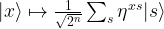
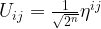
$|x \rangle \mapsto \frac{1}{\sqrt{2^n}} \sum_s \eta^{xs} |s \rangle$

where $\eta$ is an 2ⁿ-th root of unity with n being the number of qubits in the register, i.e.

$\eta = \exp \frac{2\pi i}{2^n}$

How can we effectively create this state with a quantum circuit? They key to this is the observation (see the references below) that the result of the quantum Fourier transform can be written as a product state, namely as

$\sum_s \eta^{xs} |s \rangle = (|0\rangle + \eta^{2^{n-1} x}|1\rangle)(|0 \rangle + \eta^{2^{n-2}x}|1 \rangle) \cdots (|0 \rangle + \eta^x|1 \rangle)$

which you can easily verify by multiplying out the product and collecting terms.

Here we use the tensor product order that is prescribed by OpenQASM, i.e. the most significant bit is q[n-1]. This bit is therefore given by

$|0 \rangle + \eta^{2^{n-1}x} |1 \rangle$

Let us analyse this expression further. For that purpose, we decompose x into its representation as a binary number, i.e. we write

$x = \sum_{i=0}^{n-1} 2^i x_i$

with x_i being the binary digits of x. If we now multiply this by 2^n-1, we will get $2^{n-1} x_0$ plus a multiple of 2ⁿ. As $\eta$ is a root of unity, this multiple cancels out and we obtain that

$\eta^{2^{n-1}x} = \eta^{2^{n-1}x_0} = e^{\pi i x_0} = (-1)^{x_0}$

Thus, we can write the most significant qubit of the Fourier transform as

$|0 \rangle + (-1)^{x_0} |1 \rangle$

which is nothing but

$H |x_0\rangle$

Thus we obtain the most significant qubit of the quantum Fourier transform by simply applying a Hadamard gate to the least significant qubit of the input.

This is nice and simple, but what about the next qubit, i.e. qubit n-2? From the decomposition above, we can see that this is simply

$|0 \rangle + \eta^{2^{n-2}x} |1 \rangle$

Using exactly the same arguments as for the most significant qubit, we easily find that this is

$|0 \rangle + \eta^{2^{n-2}x_0} H |x_1 \rangle$

Thus we obtain this qubit from qubit 1 by first applying a Hadamard gate and then a conditional phase gate, i.e. a conditional rotation around the z-axis, conditioned on the value of x₀. In general, qubit n-j is

$|0 \rangle + \prod_{i < j - 1} \eta^{2^{n-j+i}x_i} H |x_{j-1}\rangle$

which is a Hadamard gate followed by a sequence of conditional rotations around the z-axis, conditioned on the qubits with lower significance.

So we find that each qubit of the Fourier transform is obtained by applying a Hadamard followed by a sequence of conditional rotations. However, the order of the qubits in the output is reversed, i.e. qubit n-j is obtained by letting gates act on qubit j. Therefore, at the end of the circuit, we need to revert the order of the qubits.

In OpenQASM and Qiskit, a conditional rotation around the z-axis is called CU1, and there are swap gates that we can use to implement the final reversing of the qubits. Thus, we can use the following code to build a quantum Fourier transformation circuit acting on n qubits.

def nBitQFT(q,c,n):
    circuit = QuantumCircuit(q,c)
    #
    # We start with the most significant bit
    #
    for k in range(n):
        j = n - k
        # Add the Hadamard to qubit j-1
        circuit.h(q[j-1])
        #
        # there is one conditional rotation for
        # each qubit with lower significance
        for i in reversed(range(j-1)):
            circuit.cu1(2*np.pi/2**(j-i),q[i], q[j-1])
    #
    # Finally we need to swap qubits
    #
    for i in range(n//2):
        circuit.swap(q[i], q[n-i-1])
    return circuit

Here is the circuit that this code produces for n=4. We can clearly see the structure – on each qubit, we first act with a Hadamard gate, followed by a sequence of conditional rotations with decreasing angle, conditioned on the less significant qubits, and finally reorder the qubits.

This is already a fairly complex circuit, and we need to find a way to test it. Let us look at the options we have. First, a quantum circuit is a unitary transformation and can be described by a matrix. In our case, it is especially easy to figure out what this matrix should be. Looking at the formula for the quantum Fourier transform, we find that the matrix describing this transformation with respect to the computational basis has the elements

$U_{ij} = \frac{1}{\sqrt{2^n}} \eta^{ij}$

The Qiskit frameworks comes with a simulator called the unitary_simulator that accepts a quantum circuit as input and returns the matrix describing that circuit. Thus, one possible test approach could be to build the circuit, run the unitary simulator on it, and to compare the resulting unitary matrix with the expected result given by the formula above. In Python, the expected result is produced by the following code

def qftMatrix(n):
    qft = np.zeros([2**n,2**n], dtype=complex)
    for i in range(2**n):
        for j in range(2**n):
            qft[i,j] = np.exp(i*j*2*1j*np.pi/(2**n))
    return 1/np.sqrt(2**n)*qft

and the test can be done using the following function

def testCircuit(n):
    q = QuantumRegister(n,"x")
    c = ClassicalRegister(n,"c")
    circuit = nBitQFT(q,c,n)

    backend = Aer.get_backend('unitary_simulator')
    job = execute(circuit, backend)
    actual = job.result().get_unitary()
    expected = qftMatrix(n)
    delta = actual - expected
    print("Deviation: ", round(np.linalg.norm(delta),10))
    return circuit

The outcome is reassuring – we find that the matrices are the same within the usual floating point rounding differences.

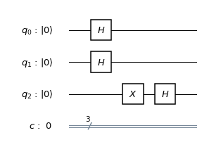
After passing this test, a next reasonable validation step could be to run the algorithm on a specific input. We know that the QFT will map the state $|0 \rangle$ into an equal superposition of all elements of the computational basis. Conversely, we therefore expect that if we start with such a superposition, the QFT will map the superposition onto $|0\rangle$ , at least up to a phase.

Let us try this out. Our test circuit will consist of a layer of Hadamard gates to create the equal superposition, followed by the QFT circuit, followed by a measurement. The resulting circuit for n=4 is displayed below.

It we run this circuit on the QASM simulator embedded into Qiskit, the result is as expected – for 1024 shots, we get 1024 times the output ‘0000’. So our circuit works – at least theoretically. But what about real hardware?

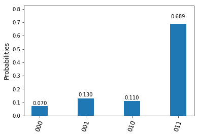
Let us compile and run the circuit targeting the IBM Q Experience 14 qubit device. If we dump the QASM code after compilation, we see that the overall circuit will have roughly 140 gates. This is already significant, and we expect to see some noise. To see how bad it is, I have conducted several test runs and plotted the results as a histogramm (if you want to play with this yourself, you will find the notebook on Github). Here is the output of a run with n=4.

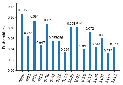
We still see a clear peak at the expected result, but also see that the noise level is close to making the result unusable – if we did not know the result upfront, we would probably not dare to postulate anything from this output. With only three qubits, the situation becomes slightly better but is still far from being satisfactory.

Of course we could now start to optimize the circuit – remove cancelling Hadamard gates, remove the final swap gates, reorder qubits to take the coupling map into account and so on – but it becomes clear that with the current noise level, we are quickly reaching a point where even comparatively simple circuit will inflict a level of noise that is at best difficult to handle. Hopefully, this is what you expected after reading my posts on quantum error correction, but I found it instructive to see noise in action in this example.

References

1. M. Nielsen, I. Chuang, Quantum Computation and Quantum Information, Cambridge University Press 2010
2. R. Cleve, A. Ekert, C. Macchiavello, M. Mosca, Quantum Algorithms revisited, arXiv:9708016

Running the Deutsch-Jozsa algorithm on IBMs Q experience

In one of the previous posts, we have looked at the basics of the Qiskit package that allows us to create and run quantum algorithms in Python. In this post, we will apply this to model and execute a real quantum algorithm – the Deutsch-Jozsa algorithm.

Recall that the Deutsch-Jozsa algorithm is designed to solve the following problem. We are given a boolean function f

$f \colon \{0,1\}^n \rightarrow \{0,1\}$

in n variables. We know that the function is either constant or it is balanced (i.e. the number of times it is zero is equal to the number of times it is equal to 1). The task is to determine which of the to properties – balanced or constant – the function f has.

The first choice that we need to make is of course a suitable function f. To keep things simple, we will use a function with two variables. Maybe the most straightforward example for a balanced function in two variables is the classical XOR function.

$f(x_0, x_1) = x_0 \oplus x_1$

Thus our first task is to develop a quantum equivalent of this function, i.e. a reversible version of f.

Recall that in general, given a boolean function f, we can define a unitary transformation U_f by the following rule

$U_f(|x \rangle |y \rangle) = |x \rangle |y \oplus f(x) \rangle$

Thus U_f flips the target qubit y if f(x) is one and leaves it unchanged otherwise. In our case, combining this with the definition of the XOR function implies that we are looking for a circuit acting on three qubits – two input qubits and one target qubit – that flips the target qubit if and only if the two input qubits are not equal. From this textual description, it is obvious that this can be constructed using a sequence of two CNOT gates.

Let us now go through the individual steps of the Deutsch-Jozsa algorithm, using the optimized version published 1997 in this paper by R. Cleve, A. Ekert, C. Macchiavello and M. Mosca (this version is also described in one of my earlier posts but is does not hurt to recap some of that). The first step of the algorithm is to prepare a superposition state

$|\psi_0 \rangle = \frac{1}{2} \sum_x |x \rangle$

This is accomplished by applying a Hadamard gate to each of the two qubits that make up our primary register in which the variable x lives. We then add an ancilla qubit that is in the state $H|1 \rangle$ , so that our state is now

$\frac{1}{2} \sum_x |x \rangle \otimes H |1 \rangle = \frac{1}{2\sqrt{2}} \sum_x |x , 0 \rangle - |x, 1 \rangle$

So far our circuit looks as follows.

Next we apply the oracle U_f to our state. According to the definition of the oracle, we have

$U_f |x, 0 \rangle = |x\rangle |f(x) \rangle$

and

$U_f |x, 1 \rangle = |x\rangle |f(x) \oplus 1\rangle$

Therefore we find that

From this formula, we can read off how U_f acts depending on the value of f(x). If f(x) is 0, the right hand side is equal to the left hand side and U_f acts trivially. If, however, f(x) is one, the right hand side is simply minus the left hand side, and U_f acts as multiplication by -1. Combining this with our previous formula, we obtain

$U_f \colon: \frac{1}{2} \sum_x |x \rangle \otimes H |1 \rangle \mapsto \frac{1}{2} \sum_x (-1)^{f(x)}|x \rangle \otimes H |1 \rangle$

Next, we apply again the Hadamard operator followed by the Pauli X gate to the third qubit (the ancilla), i.e. we uncompute the ancilla qubit. From the expression above, we can read off directly that the result left in the first two qubits will be

$|\psi \rangle = \frac{1}{2} \sum_x (-1)^{f(x)}|x \rangle$

This is the vector that we will have in the first two qubits of our quantum register when we have processed the following circuit.

Let us now calculate the overlap, i.e. the scalar product, between this vector and the initial superposition $|\psi_0 \rangle$ . Clearly,

$\langle \psi_0 |\psi \rangle = \frac{1}{4} \sum_x (-1)^{f(x)}$

We find that this overlap is zero if and only if the function f is balanced. But how can we measure this scalar product? To see this, recall that the initial state $|\psi_0 \rangle$ is the result of applying the tensor product H² of the two Hadamard operators to the first two qubits in the fiducial state. Thus we can write our scalar product as

$\langle \psi_0 |\psi \rangle = \langle 0 | H^2 |\psi \rangle = \langle 0 | H^2 \psi \rangle$

In other words, we can determine the scalar product by again applying a Hadamard operator to each of the first two qubits and measuring the overlap of the resulting state with the basis state $|00 \rangle$ which is the same thing as the probability to measure $|00 \rangle$ when we perform a measurement in the computational basis. Thus we finally obtain the following circuit

and the function f is balanced if and only if the probability to measure $|00 \rangle$ is zero.

Let us now turn this into Python code using Qiskit. I found it useful to create subroutines that act on a given circuit and build parts of the circuit which can then be tested independently from each other on a simulator before combining them. Here is the code to create the oracle for our balanced function f.

def createOracleBalanced(q,c):
    circuit = QuantumCircuit(q,c)
    circuit.cx(q[0], q[2])
    circuit.cx(q[1], q[2])
    circuit.barrier(q)
    return circuit

Similarly, we can write routines that create the initial state and join the ancilla qubit.

def createInitialState(circuit):
    circuit.h(q[0])
    circuit.h(q[1])
    circuit.barrier(q)

def addAncilla(circuit):
    circuit.x(q[2])
    circuit.h(q[2])
    circuit.barrier(q)

Finally, we need to be able to uncompute the ancilla and to add the final measurements.

def uncomputeAncilla(circuit):
    circuit.h(q[2])
    circuit.x(q[2])
    circuit.barrier(q)

def addMeasurement(circuit):
    circuit.h(q[0])
    circuit.h(q[1])
    circuit.barrier(q)
    circuit.measure(q[0], c[0])
    circuit.measure(q[1], c[1])
    circuit.barrier(q)

A word on barriers. In this example code, we have added barriers after each part of the circuit. Barriers are an element of the OpenQASM specification and instruct the compiler not to combine gates placed on different sides of a barrier during optimization. In Qiskit, barriers have the additional benefit of structuring the visualization of a circuit, and this is the main reason I have included them here. In an optimized version, it would probably be safe to remove them.

After all these preparations, it is now easy to compile the full circuit. This is done by the following code snippet – note that we can apply the + operator to two circuits to tell Qiskit to concatenate the circuits.

q = QuantumRegister(3,"q")
c = ClassicalRegister(3,"c")
circuit = QuantumCircuit(q,c)
createInitialState(circuit)
addAncilla(circuit)
circuit = circuit + (createOracleBalanced(q,c))
uncomputeAncilla(circuit)
addMeasurement(circuit)

We can then compile this code for a simulator or a backend as explained in my last post on the IBM Q experience (you can also find the full source code here). The following histogramm shows the result of the final measurement after running this on the ibmqx4 5 qubit quantum computer.

We see, as in the experiments conducted before, that the theoretically expected result (confirmed by running the circuit on a simulator) is blurred by noise – we get the value 00 in a few instances, even though the function is balanced. Even though the outcome can still be derived with a reasonable likelihood, we start to get a feeling for the issues that we might have with noise for more complex functions and circuits.

It is instructive to extract the compiled QASM from the resulting qobj and load that code into the IBM Q Experience composer. After a few beautifications, the resulting code (which you can get here) is displayed as follows in the composer.

If we compare this to the original circuit, we see that the compiler has in fact rearranged the CNOT gates that make up our oracle. The reason is that the IBMQX4 device can only realize specific CNOT gates. It can, for instance, implement a CNOT gate with q[1] as control as q[0] as target, but not vice versa. Therefore the compiler has added Hadamard gates to swap control and target qubit. We also see that the compiler has respected the barriers and not cancelled some of the double Hadamard gates. If we remove the barriers and remove all Hadamard gates that clearly cancel each other, we finally obtain a greatly simplified version of the circuit which looks as follows.

Of course this simplification hinges on the special choice of the function f. Nevertheless, it is useful – fewer gates mean fewer errors. If we compare the error rates of the optimized circuit with the new circuit, we find that while the original version had an error (i.e. an unexpected amplitude of $|00 \rangle$ ) of roughly 10%, a run with the optimized circuit showed an error of only 5,5%.

This completes our post. The next algorithm that we will implement is Shor’s algorithm and the quantum Fourier transform.

Quantum error correction with stabilizer codes

In our previous discussion of quantum error correction, we have assumed that quantum gates can act on any two physical qubits. In reality, however, this is not true – only nearby qubits and interact, and our error correction needs to take the geometric arrangements of the qubits into account. The link between these geometric constraints and the theory of quantum error correction is the stabilizer formalism described first in [2].

This post will be a bit more formal, but is a necessary preparation to be able to define and understand the surface code and other topological codes. To introduce and motivate the formalism, let us for a moment come back to the simple example studied before – the three-bit code. In this code, the logical states were

$|0 \rangle_L = |000 \rangle$

and

$|1 \rangle_L = |111 \rangle$

These logical states span our two-dimensional code space and describe one logical qubit. A single bit flip error will flip one of the three involved qubits. Suppose, for instance, that a bit flip occurs on the first or second qubit. This error will modify our logical states as follows (the first two lines represent a bit flip on the first qubit, the next two lines a bit flip on the second qubit

$|0 \rangle_L \mapsto |100 \rangle$

$|1 \rangle_L \mapsto |011 \rangle$

$|0 \rangle_L \mapsto |010 \rangle$

$|1 \rangle_L \mapsto |101 \rangle$

Now consider the operator

$M_1 = \sigma_z^1 \sigma_z^2$

where the upper index on a Pauli matrix indicates the qubit on which the operator acts. The error-free logical states are both eigenstates of this operator with eigenvalue +1. The states that result out of a bit-flip error are also eigenstates of this operator, but with eigenvalue -1. Thus, a measurement of this operator will tell us whether a bit flip on the first or second qubit has occurred. Similarly, to also detect a bit flip on the third qubit, we need a measurement for a second operator, namely

$M_2 = \sigma_z^1 \sigma_z^3$

Let us now write down a few properties of these operators. First, they are hermitian and therefore correspond to measurements. Second, the logical states are eigenvectors of these operators with eigenvalues +1 and the code space is exactly the subspace of the three-qubit state space that is fixed by M₁ and M₂. We can think of these operators as defining linear constraints that together define the code space, as indicated below.

Moreover, if a bit flip error occurs, the resulting state will again be an eigenvalue, but for at least one of the operators the new eigenvalue will be -1. Thus, errors correspond to violated constraints. Finally, the two operators commute and can therefore be measured simultaneously.

These properties allow us to express the three bit code entirely in terms of the operators M₁ and M₂. The code space is the subspace which is left invariant by these operators. The syndrome measurement can be done by measuring both operators simultaneously, which is possible because they commute. Finally, all involved states – code space and states after bit flip errors – are eigenstates and therefore the measurement process does not collapse a superposition of these states and can therefore be executed without interfering with the actual quantum algorithm that we want to run.

This correspondence between sets of operators – the M_i in our case – and quantum error correction is the core of the stabilizer formalism. In a more general setting, we are looking at the Hilbert space of dimension 2ⁿ spanned by n physical qubits. Products of n Pauli matrices (where we include the identity matrix) are acting on this Hilbert space and form a group ${\mathcal G}_n$ called the Pauli group. Put differently, the Pauli group consists of those linear operators on the Hilbert space that can be written as a product

$g = \mu (\sigma_x^1)^{a_1} (\sigma_y^1)^{b_1} (\sigma_z^1)^{c_1}\cdots (\sigma_x^n)^{a_n}(\sigma_y^n)^{b_n} (\sigma_z^n)^{c_n}$

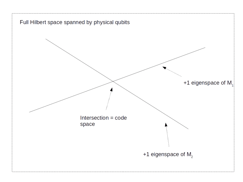
with coefficients $a_i, b_ic, c_i$ and an overall phase factor $\mu \in \{ \pm 1, \pm i \}$ (we can even assume that all the $b_i$ are equal to one as $\sigma_x \sigma_z$ is a multiple of $\sigma_y$ ). Any two elements of the Pauli group either commute or anti-commute. Within this group, we now consider a finite set $\{ M_i \}$ of commuting elements and the subgroup S of the Pauli group generated by this set. This group (which is abelian as it is generated by mutually commuting elements) is called the stabilizer group. To this group, we can associate the subspace that consists of all vectors that are fixed by all elements of the group, i.e. the space

$T_S = \{ |\psi \rangle \, \text{such that} \, s|\psi \rangle = |\psi \rangle \forall s \in S \}$

This space will be the code space of our code. If the group S is generated by l independent generators, the dimension of the code space can be seen to be 2^n-l.

In the example of the three bit code, we had n=3 and l=2, which gives us a two-dimensional code space, corresponding to one logical qubit (if you try work out the details, you will see that in order for this to be true, we have to assume that $-1 \notin S$ – you might want to take a look at my notes or the chapters on quantum error correction in [1] for the mathematical details).

Which errors is our code able to detect? Suppose that E is an error operator that is itself in the Pauli group. We know that any two elements of the Pauli group either commute or anti-commute. Let us assume that E does in fact anti-commute with some element s of S. If $|\psi \rangle$ is a state in the code space, we can then calculate

$s E |\psi \rangle = - E s |\psi \rangle = - E |\psi \rangle$

Therefore the state $E |\psi \rangle$ is now in the -1 eigenspace of s. Thus if we measure all elements of S, the outcome -1 for one of the measurements will tell us that an error has occurred. A similar argument shows that if the product of any two errors anti-commutes with at least one element of S, then we can also correct the error based on only the measurement results of elements in S. Mathematically speaking, the set of all elements of the Pauli group that commute with all elements of S is the centralizer of S, which in this case turns out to be equal to the normalizer N(S) of S, and a set $\{E_\alpha \}$ of errors can be detected and corrected if and only if

$E_\alpha E_\beta \in S \cup (\mathcal{G} - N(S))$

for any two error operators $E_\alpha, E_\beta$ . So the elements of the Pauli group that are neither in S nor in N(S) correspond to correctable errors.

What do the elements of the normalizer correspond to? Suppose that n is an element in the normalizer and therefore commutes with all elements of S. Then, for any element s in S and any element $|\psi \rangle$ of the code space, we have

$s n |\psi \rangle = n s |\psi \rangle = n |\psi \rangle$

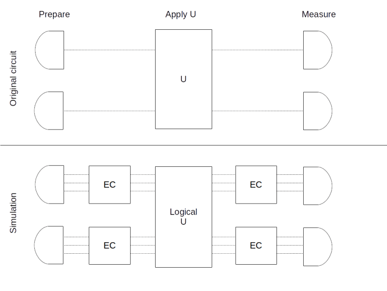
Consequently, the element $n |\psi \rangle$ is again fixed by all elements of S and therefore in the code space T_S. Thus the elements of N(S) generate automorphisms of the code space, i.e. logical operations. It is one of the strengths of the stabilizer formalism that once we have the stabilizer group S, we can not only derive the code space and the correctable errors, but can also use group theoretic considerations to describe logical operations – this will become clearer as we study surface codes in a later post.

For later reference, let us briefly summarize what we have found. Given l independent generators s_i of the stabilizer S, we can define a code space as the set of all vectors that are fixed by the s_i. This subspace will encode n – l logical qubits in n physical qubits. To detect an error, we measure all the s_i. Each measurement will give us minus one or plus one. Any occurrence of minus one indicates an error (this is why the combined result of all measurements is usually called the error syndrome) and will also tell us which operation we have to apply to correct the error. To implement logical quantum gates on our code space, we can apply elements in the normalizer N(S) that map the code space into itself. Thus we have expressed error detection, error correction and logical operations entirely in terms of the stabilizer group and the language of group theory.

But how do we find useful stabilizer codes? One approach is given by the check matrix formalism, which allows us to express stabilizer codes in terms matrices and metrics, i.e. in terms of linear algebra. This approach is generalizing the parity check matrix from the classical theory of error correction. A second source of stabilizers, however, comes from a more surprising direction – algebraic topology. In fact, given a surface described in terms of a cell complex, we can associate elements of the Pauli group with every cycle and every co-cycle. For certain choices of cycles and cocycles, this will give us abelian subgroups of the Pauli group which in turn create error correction codes. This is how geometrical constraints in the actual implementation enter the scene and leads to a class of codes known as surface codes and toric codes that we will start to study in my next post.

1. E. Rieffel, W. Polak, Quantum computing – a gentle introduction, MIT Press, Cambridge 2011
2. D. Gottesman, Stabilizer Codes and Quantum Error Correction, Caltech Ph.D. Thesis, available as arXiv:quant-ph/9705052
3. J. Kempe, Approaches to quantum error correction, S\’eminaire Poincar\’e 1 (2005), pp. 65–93, available as arXiv:quant-ph/0612185

Fault tolerant quantum computing

In the previous post, we have looked at the basic ideas behind quantum error correction, namely the encoding of logical states so that we are able to detect and correct errors like bit flip and phase flip errors. Unfortunately, this is not yet good enough to implement quantum computing in a fault-tolerant way.

What is still missing? First, we have only discussed errors that impact saved quantum states, i.e. random bit flips or phase flips that invalidate a given state stored in a quantum register. We have not yet, however, understood how we can protect quantum states during processing, i.e. deal with errors that do not occur on a saved qubit but that occur while we manipulate these qubits by executing quantum gates.

Second, and maybe even worse, implementing error correction involves adding additional qubits and quantum gates to our circuit. Obviously, these additional elements will again be subject to errors and require protection. So we might need an additional correction step to account for these errors. This additional step will again introduce additional errors and so forth. It is not a priori clear that we do not introduce more errors than we can correct when following this path. Fortunately, the famous threshold theorem asserts that under certain conditions, we can win this race and correct errors faster than we create them.

Error propagation and transversal quantum gates

But let us start with the first question – how can we implement quantum gates in a fault tolerant way? To illustrate the challenge, we start with a simple (though unrealistic) example. Suppose that we wanted to perform a CNOT gate on two states encoded with the three-bit code. The obvious approach – decode the two input states, apply an ordinary CNOT and encode again – does not appear to be a good choice, as uncontrolled errors might sneak in while the states are unencoded and therefore vulnerable. So let us try to implement a CNOT operation directly on the encoded states. This can be done with the following circuit.

Let us see why this circuit works. Suppose the control word is the encoded (logical) state

$|0 \rangle_L = |000 \rangle$

Then all three qubits in the control word are zero. Consequently, the three CNOT gates do nothing and the target word is not changed. If, on the other hand, the control word is

$|1 \rangle_L = |111 \rangle$

then all three qubits in the target word will be toggled, and thus the target word $|0 \rangle_L$ will be mapped to $|1\rangle_L$ . Thus our circuit does in fact implement a CNOT gate on the logical level.

However, there is a problem with this circuit. To see this, suppose that there is a bit flip error in the first qubit of the control word. Then this error will make all three CNOT gates toggle their target state, and a logical $|0 \rangle_L$ on the target qubits will be flipped into a logical $|1 \rangle_L$ . Thus even a single error in the input will render the result unusable. This is an example for uncontrolled error propagation: a single error in the control word input has propagated across all three qubits that make up the second input and our code – which is only able to protect against single qubit errors – fails.

Obviously, the propagation of errors can never be entirely avoided. However, what we can avoid is the uncontrolled propagation. To explain this, let us take a look at the following circuit.

This circuit also realizes a CNOT on the level of logical states. However, for this circuit, an error in one of the qubits of the block of three qubits that encode the logical control bit can only propagate into one qubit in the second block – the block of three qubits that encode the target bit. Therefore one error per input block will only propagate into one error in each output block. If we are able to fully recover from one qubit errors per block, we can detect and correct the errors even though they have propagated through the circuit (again as long as only one error occurs). Thus the trick is to somehow spread potential errors across multiple blocks so that no single block is fully corrupted. This connectivity property of a circuit is sometimes called transversality.

Transversal gates are fault-tolerant, as an error in one qubit can only propagate into one qubit of any other code block, a situation from which we can recover. For many codes, many basic gates can be implemented qubit-wise and therefore transversally on the level of logical qubits. Unfortunately, a full set of universal quantum gates cannot be constructed in such a way – typically one gate remains for which no transversal implementation can be found. Fortunately, there are other (considerably more complicated) methods available to construct fault-tolerant logical gates. In [1], Shor has described the first fully universal set of fault-tolerant logical gates for his nine qubit code. In many modern implementations, a class of codes called surface codes are used, that also allow us to implement a universal set of quantum gates in a fault tolerant way and that we will study in a later post. Similar approaches work for measurements that can have errors as well and that need to be organized in a way so that errors can be detected and corrected, and the same applies for the actual error correction circuits.

Fault tolerant quantum computation and the threshold theorem

Even if we are able to implement quantum gates in a fault tolerant way, one challenge remains. So far, we have only discussed how to protect against single qubit errors. Of course, the rationale behind this was the assumption that errors in two or more qubits are much less probable than single qubit errors. Thus, we have reduced the error probability. For real applications, our new, reduced error probability might still not be sufficient. We therefore might have to add additional error correction circuits. Now the probability of failure for a circuit is not only a function of the reliability of every single component, but also a function of the number of components. The more error correction mechanisms we add, the higher the number of components and the higher the overall fault probability. In the worst case, the increase of the fault probability by adding the additional components needed for the error correction might eat up all the benefits of the error correction and lead to an overall higher probability of failure.

To be able to better grasp the problem, let us introduce some terminology. Suppose we are given a circuit C that describes a quantum computation. We can think of the overall computation as being organized in individual time steps. At each time step, every qubit in the circuit takes part in a basic set of possible operations (or, to mention a different term that is sometimes used, locations). This can be a gate, the preparation of a qubit in a initial state, a measurement or a “wait step”, i.e. the identity operation leaving the involved qubits unchanged. At each time step, a qubit is involved in exactly one of these operations.

Given such a circuit, we can now try to build a fault tolerant circuit performing the same computation as follows. We replace each qubit in the circuit C by a block of qubits encoding a logical qubit. Similarly, we replace each operation in C by the corresponding fault tolerant equivalent, i.e. we replace each gate by the corresponding logical gate, a measurement by a fault tolerant measurement, and a preparation by a fault tolerant state preparation. In addition, we place a (fault tolerant) error correction circuit in each block which is the output of a logical gate. The result is called a simulation of the original circuit. An example is displayed below, using (roughly) the graphical language described in [2].

The upper part of this diagram shows an original circuit, in which we prepare two qubits in a known state, then apply the unitary transformation U and finally measure both qubits. The result of the replacement procedure described above is displayed in the lower part of the picture, using again the (unrealistic) example of a three qubit code. Here we have replaced each qubit by a corresponding block of three qubits holding the code word. The operation U has been replaced by its logical implementation, acting on the encoded states, and both after the preparation and after applying U, we add a circuit performing error correction.

Let us now study how the fault probability changes when we pass to a simulation. In general, this is a long and complicated argument, and we refer the reader to [3], [4] and [5] for the details. However, there is a simple example that can be used to illustrate some of the key ideas.

In fact, let us go back to the circuit above that we have used for a fault-tolerant implementation of the CNOT gate. To analyze the probability that this circuit fails, let us assume that the only error that can occur is a bit flip error in the target qubit of each physical CNOT gate and that this error occurs with probability p. Thus we assume that error correction, state preparation and measurement work in an idealized, error free way.

Let us now look at the different combinations of faults that can occur during a specific run of the simulation circuit, i.e. a different fault paths. A first fault path is given by a single bit flip error in one of the target qubits after executing the CNOT operation. However, this affects only one qubit and can therefore be corrected by the error correction circuit. Thus, for this fault path, the simulation works correctly.

There is, however, a different fault path, given by a fault in target qubit one and target qubit two, whereas the CNOT acting on target qubit three operates correctly. Assuming that the individual faults are statistically independent, the probability for this fault path is

$p \cdot p \cdot (1 - p) = p^2 - p^3$

This would introduce an error from which we could not recover, as our code is only able to correct errors in one qubit. But this is not yet the overall probability of failure for our new circuit, as there is a second fault path that we need to consider – we could as well have a failure in the first and the third instead of the first and second qubit. Obviously, the probability for this fault path is the same. And there is a third fault path with two errors, given by an error in the second and third target qubit. These three different fault paths, all with two errors, correspond to the

${{3} \choose {2}} = 3$

possibilities to choose two error locations out of the three target qubits. And finally, it might happen that faults occur in all three locations, an event which clearly has probability p³. Thus the overall probability to have at least two faults is

$3 (p^2 - p^3) + p^3 = 3 p^2 - 2 p^3 \leq 3 p^2$

Thus the overall probability that the circuit does not operate correctly does not reduce from p – for the physical CNOT operation without error protection – to p², but to 3 p², where the factor 3 reflects the growth of the circuit when passing from the physical circuit to the simulation, i.e. the impact of the additional gates.

Of course this is a very simplified example, but the hard work done in the original papers in the references demonstrates that the result is true in general: if we pass from a circuit to its simulation, the change of the error rate is described by a rule of the form

$p \mapsto c p^{t+1}$

where c is a constant that reflects the growth of the circuit and t is the number of errors that the code that we use can still correct. Obviously, this does not help unless the right hand side is smaller than the left hand side, i.e. unless p is smaller than a threshold given by

$p < c^{-\frac{1}{t}} = p_{crit}$

If this is true, we can even iterate the procedure, and reduce the error rate below every prescribed level by adding additional layers of simulation. Thus given physical operations with error rate less than p_crit, we can implement each quantum circuit in a fault-tolerant way with arbitrary reliability.

Unfortunately, the exact value of the threshold is not known. The initial estimate provided in [3] was in the range of 10^-6. Later, this was improved by several authors, and is mostly assumed to be in the range between 10^-4 and 10^-2 (see [6] for an overview of some results in this direction).

As c is in the order of p_crit^-t, this implies that we need as many as a few hundred to a few thousand physical gates and qubits to simulate one logical qubit. Note that in general, the overhead depends on the desired accuracy and the level of simulations needed as well as on the factors entering the constant c, i.e. the encoding, the architecture of the logical gates, as well as how close the actual physical error rate is to the threshold. Improving the threshold and thereby reducing the overhead remains one of the most active areas of current research in quantum computing and is essential for paving the road towards a large-scale fully fault tolerant universal quantum computer.

At the time of writing, a class of codes known as surface codes appear to be good candidates for the implementation of fault-tolerant quantum computers, not only because these codes have good error correction properties, but also because they are well adapted to the geometry of the actual quantum computer. In the next few posts, we will work towards understanding surface codes and other topological codes, starting with the formalism of stabilizer codes that will be the focus of the next post.

1. P. Shor, Scheme for reducing decoherence in quantum computer memory, Phys. Rev. A Vol. 52 (1995) Issue 4, pp. 2493–2496
2. D. Gottesman, An Introduction to Quantum Error Correction and Fault-Tolerant Quantum Computation, arXiv:0904.2557v1
3. D. Arahonov, M. Ben-Or, Fault Tolerant Quantum Computation with Constant Error, arXiv:quant-ph/9611025
4. E. Knill, R. Laflamme, W.H. Zurek, Threshold accuracy for quantum computation, arXiv:quant-ph/9610011,
5. P. Aliferis, D. Gottesman, J. Preskill, Quantum accuracy threshold for concatenated distance-3 codes, arXiv:quant-ph/0504218v3
6. S. J. Devitt, W. J. Munro, K. Nemoto, Quantum Error Correction for Beginners, arXiv:0905.2794v4