In my recent post on Hopfield networks, we have seen that these networks suffer from the problem of spurious minima and that the deterministic nature of the dynamics of the network makes it difficult to escape from a local minimum. A possible approach to avoid this issue is to randomize the update rule. Intuitively, we want to move into a direction of lower energy most of the time, but sometimes allow the network to move a different direction, so that there is a certain probability to move away from a local minimum.
In a certain sense, a Boltzmann machine is exactly this – a stochastic version of a Hopfield network. If we want to pursue the physical analogy further, think of a Hopfield network as an Ising model at a very low temperature, and of a Boltzmann machine as a “warm” version of the same system – the higher the temperature, the higher the tendency of the network to behave randomly and to escape local minima. As for the Hopfield network, there are different versions of this model. We can allow the units to take any real value, or we can restrict the values to two values. In this post, we will restrict ourselves to binary units. Thus we consider a set of N binary units, taking values -1 and +1, so that our state space is again

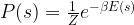
Similar to a Hopfield network, each unit can be connected to every other unit, so that again the weights are given by an N x N matrix W that we assume to be symmetric and zero along the diagonal. For a state s, we define the energy to be

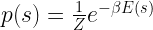
This energy defines a Boltzmann distribution on the state space, given by
Now our aim is to adjust the weights such that this distribution is the best possible approximation to the real distribution behind the training data.
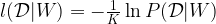
How do we measure the distance between the current distribution and the target distribution? A common approach to do this is called the maximum likelihood approach: given a set of weights W, we try to maximize the probability for the training data under the distribution given by W. For convenience, one does usually not maximize this function directly, but instead minimizes minus the logarithm of this probability, divided by the number K of samples. In our case, we therefore try to minimize the loss function
Now let us assume that our sample is given by K data points that we denote by ![s^{(k]}](https://s0.wp.com/latex.php?latex=s%5E%7B%28k%5D%7D&bg=FFFFFF&fg=000&s=0&c=20201002)

Using the definition of the Boltzmann distribution and the partition function Z, we can therefore express our loss function as

where 
Now how do we minimize this function? An obvious approach would be to use the gradient descent algorithm or one of its variants. To be able to do this, we need the gradient of the loss function. Let us first calculate the partial derivative for the first term, the logarithm of the partition function. This is

Now the sum on the right hand side of this equation is of the form “probability of a state times a function of this state”. In other words, this is an expectation value. Using the standard notation for expectation values, we can therefore write

If you remember that expectation values can be approximated using Monte Carlo methods, this is encouraging, at least we would have an idea how to calculate this. Let us see whether the second term can be expressed as an expectation values as well. In fact, this is even easier.
Now this is again an expectation value – it is not an expectation value under the model distribution (the Boltzmann distribution) but under the empirical distribution of the data set.

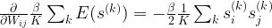
Finally, our expression for the first term still contains the derivative of the energy, which is easily calculated. Putting all of this together, we now obtain a formula for the gradient of the loss function which is maybe the most important single formula for Boltzmann machines that you need to remember.
![\frac{\partial}{\partial W_{ij}} l({\mathcal D} | W) = - \frac{\beta}{2} \left[ \langle s_i s_j \rangle_{\mathcal D} - \langle s_i s_j \rangle_P \right]](https://s0.wp.com/latex.php?latex=%5Cfrac%7B%5Cpartial%7D%7B%5Cpartial+W_%7Bij%7D%7D+l%28%7B%5Cmathcal+D%7D+%7C+W%29+%3D+-+%5Cfrac%7B%5Cbeta%7D%7B2%7D+%5Cleft%5B+%5Clangle+s_i+s_j+%5Crangle_%7B%5Cmathcal+D%7D+-+%5Clangle+s_i+s_j+%5Crangle_P+%5Cright%5D++&bg=FFFFFF&fg=000&s=1&c=20201002)
When using the standard gradient descent algorithm, this expression for the gradient leads to the following update rule for the weights, where 
![\Delta W_{ij} = \frac{1}{2} \lambda \beta \left[ \langle s_i s_j \rangle_{\mathcal D} - \langle s_i s_j \rangle_P \right]](https://s0.wp.com/latex.php?latex=%5CDelta+W_%7Bij%7D+%3D+%5Cfrac%7B1%7D%7B2%7D+%5Clambda+%5Cbeta+%5Cleft%5B+%5Clangle+s_i+s_j+%5Crangle_%7B%5Cmathcal+D%7D+-+%5Clangle+s_i+s_j+%5Crangle_P+%5Cright%5D++&bg=FFFFFF&fg=000&s=1&c=20201002)
Let us pause for a moment and reflect what this formula tells us. First, if we have reached our goal – model distribution and sample distribution are identical – the gradient is zero and the algorithm stops.
Second, the first term is essentially the Hebbian learning rule that we have used to train our Hopfield network. In fact, this is the weighted sum over the product 
The third point that we can observe is a bit more subtle. To explain it, assume for a moment that the data has been normalized (which is very often done in actual applications) so that its average is zero, in other words such that the expectation values

of the coordinates are all zero. For the Boltzmann distribution, this will be the case anyway as the distribution is symmetric in s (and it would therefore not even make sense to try to achieve convergence with unnormalized data). Thus the two terms that appear in the above equation are simply the elements of the covariance matrix under empirical and model distribution. This implies that a Boltzmann machine is not able to distinguish two distributions that have the same second moments as the covariance matrix is all that it sees.
That is a bit disappointing as it limits the power of our model significantly. But this is not the only problem with Boltzmann machines. Whereas we could easily calculate the first term in our formula for the weight change, the second term is more difficult. In our discussion of the Ising model, we have already seen that we could use Gibbs sampling for this, but would need to run a Gibbs sampling chain to convergence which can easily take one million steps or more for large networks. Now this is embedded into gradient descent which is by itself an iterative algorithm! Imagine that one single gradient descent step could take a few minutes and then remember that we might need several thousand of these steps and you see that we are in trouble.
Fortunately, help is on the way – with a slightly simplified model called restricted Boltzmann machines, both problems can be solved. I will look at this class of networks in my next post in this series. If you do not want to wait until then, you can take a look at my notes on Boltzmann machines that also give you some more background on what we have discussed in this post.
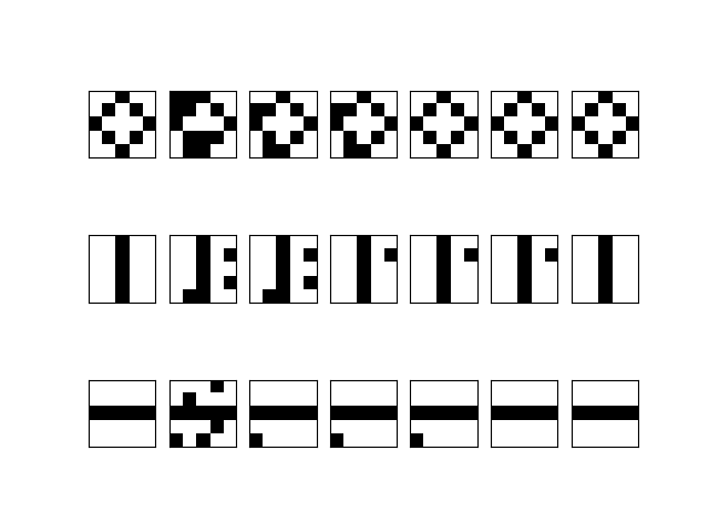
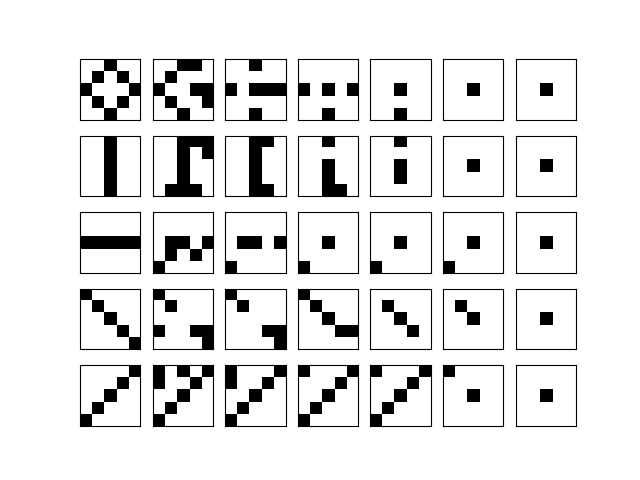
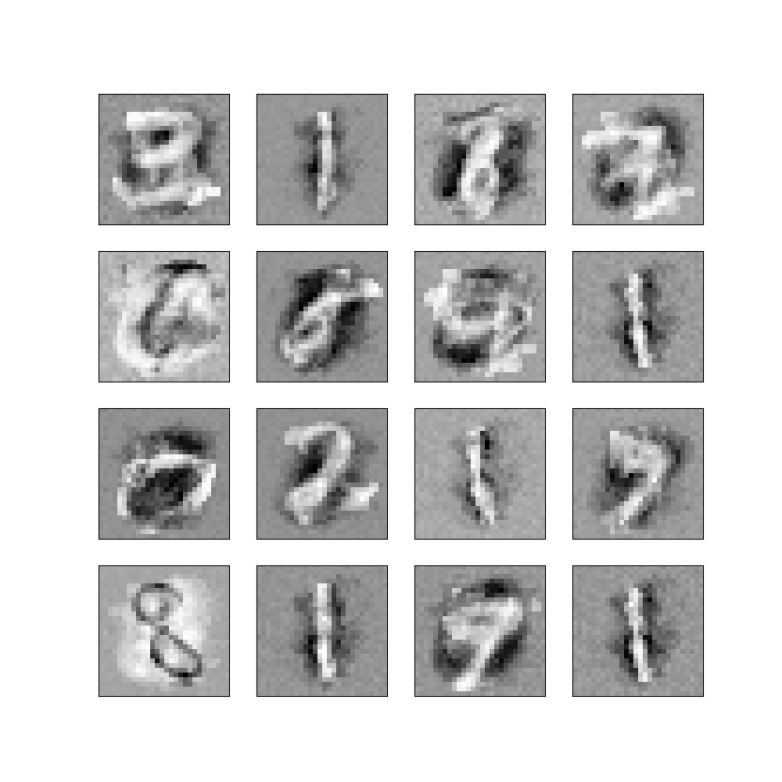
Before we close, let me briefly describe what we could do with a Boltzmann machine if we had found a way to train it. Similar to a Hopfield network, Boltzmann machines are generative models. Thus once they are trained, we can either use them to create samples or to correct errors. If, for instance, each unit corresponds to a pixel in an image of a handwritten digit, we could sample from the model to obtain artificially created images that resemble handwritten digits. We could also use the network for pattern completion – if we have an image where a few pixels have been erased, we could start the network in the state given by the remaining pixels and some random values for the unknown pixels and hope that it converges to the memorized state, thus reconstructing the unknown part of the picture. However, specifically for restricted Boltzmann machines, we will see that an even more important application is to be used as feature extractor in deep layered networks.
So there are good reasons to continue analyzing these networks – so join me again in my next post when we discuss restricted Boltzmann machines.


 patterns, where N is the number of units. In our case, with 25 units, this would be approximately 3 to 4 patterns.

 .
. is the strength of the connection between the units i and j. We assume that no neuron is connected to ifself, i.e. that
  , and that the matrix of weights is symmetric, i.e. that
  .
.

 . Let
. Let


 and the activation of unit i is never negative, this implies that during the upgrade process, the energy function will always increase or stay the same. Thus the state will settle in a local minimum of the energy function.

 is close to infinity. If the activation of unit i is positive, the probability will be very close to one. The Gibbs sampling rule will then almost certainly set the spin to +1. If the activation is negative, the probability will be zero, and we will set the spin to -1. Thus the update role of a Hopfield network corresponds to the Gibbs sampling step for an Ising model at temperature zero.
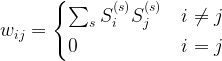
 are the states that the network should remember (in a later post in this series, we will see that this rule can be obtained as the low temperature limit of a training algorithm called contrastive divergence that is used to train a certain class of Boltzmann machines).
 and
and  have the same sign, i.e. are in the same state. This corresponds to a rule known as Hebbian learning rule that has been postulated as a principle of learning by D. Hebb and basically states that during learning, connections between neurons are enforced if these neurons fire together (

 where a value of +1 is interpreted as “spin up” and a value of -1 as “spin down”.

 (i.e. we exclude self-interactions).
 represents the external field acting on the particle at position j. The matrix J represents the interactions between the particles. In Isings original model, only nearby particles interact. In two dimensions, for instance, we think of the particles as being located on a grid and each particle has four neighbors: the particles immediately above and below it and the particles on the left and on the right. We can define a model which has a boundary or we can think of the grid as being toroidal, i.e. wrapping around.
 different states, which is roughly
  . Comparing this to the estimated age of the universe in seconds (
 , see for instance
  , will provide a good approximation for the real value. This approach is sometimes called Monte Carlo integration and the workhorse of computational statistical mechanics.
 denotes the i-th row of the matrix J and the brackets denote the ordinary scalar product. With this expression, a single Gibbs sampling step now proceeds as follows, given a state s.
 using the formula above
 if particles i and j are neighbors and zero otherwise, and also set the magnetic field to zero. The Gibbs sampling algorithm as outlined above is straightforward to implement in Python. You can get my code from GitHub as follows.
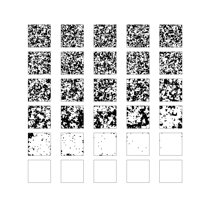

 .
. .
.


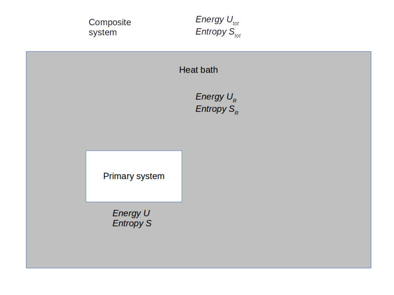
 , its entropy by
  , the energy of the heat bath by
  and the entropy of the heat bath by
  (if energy and entropy are new concepts for you, I recommend my short
  . Let us denote the number of states of the heat bath with that energy by
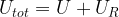
 denote the number of states of the composite system with energy
  , because every such state combines with s to an admissible state of the composite system. If all these states are equally likely, the probability for s is therefore just the fraction of these states among all possible states of the composite system, i.e.
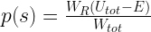

![W_{tot} = \exp \frac{1}{k} \left[ S(U) + S_R(U_{tot} - U) \right]](https://s0.wp.com/latex.php?latex=W_%7Btot%7D+%3D+%5Cexp+%5Cfrac%7B1%7D%7Bk%7D+%5Cleft%5B+%C2%A0+%C2%A0S%28U%29+%2B+S_R%28U_%7Btot%7D+-+U%29+%C2%A0+%C2%A0%5Cright%5D++&bg=FFFFFF&fg=000&s=1&c=20201002)
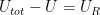 . The first derivative of the entropy with respect to the energy is – by definition – the inverse of the temperature:
 of the reservoir. In fact, we have

![p(s) = \exp \frac{1}{kT} \left[ (U - TS(U)) - E(s) \right]](https://s0.wp.com/latex.php?latex=p%28s%29+%3D+%5Cexp+%5Cfrac%7B1%7D%7BkT%7D+%5Cleft%5B+%28U+-+TS%28U%29%29+-+E%28s%29+%5Cright%5D++&bg=FFFFFF&fg=000&s=1&c=20201002)
 is the Helmholtz energy
  . If we also introduce the usual notation
  , we finally find that


 , as follows.
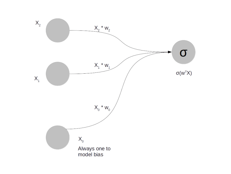
 is a function called the activation function and
  is the vector that is formed by
  and
and  . There are a few standard choices for the activation function, a common one being the
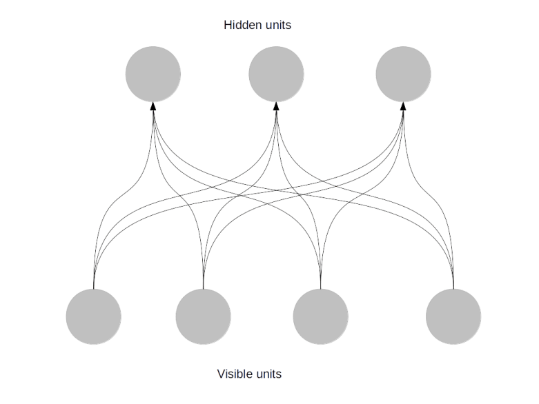

 . Even if we cannot find an analytic expression for this, we can try to approximate it. Your first idea might be “Riemann sums”, but it turns out that this is not a good idea, as our function lives in the space of all weights which has a very high dimension. Instead, we will use an approach called Monte Carlo integration where we represent the integral as an expectation value, draw a sample and approximate the expectation value by the sample average. This is where stochastical methods like Markov chains will come into play. And finally we will see that the behaviour of our network during training has some striking analogies with the behaviour of certain physical systems like solids exposed to a magnetic field at low temperatures, which are described by a model called the Ising model, and learn how techniques that physicists have developed for this type of problems apply to neuronal networks.

