OpenStack Neutron – handling instance metadata

Not all cloud instances are born equal. When a cloud instance boots, it is usually necessary to customize the instance to some extent, for instance by adding specific SSH keys or by running startup scripts. Most cloud platforms offer a mechanism called instance metadata, and the implementation of this feature in OpenStack is our topic today.

The EC2 metadata and userdata protocol

Before describing how instance metadata works, let us first try to understand the problem which this mechanism solves. Suppose you want to run a large number of Ubuntu Linux instances in a cloud environment. Most of the configuration that an instance needs will be part of the image that you use. A few configuration items, however, are typically specific for a certain machine. Standard data use cases are

  • Getting the exact version of the image running
  • SSH keys which need to be injected into the instances at boot time so that an administrator (or a tool like Ansible) can work with the machine
  • correctly setting the hostname of the instance
  • retrieving information of the IP address of the instance to be able to properly configure the network stack
  • Defining scripts and command that are executed at boot time

In 2009, AWS introduced a metadata service for its EC2 platform which was able to provide this data to a running instance. The idea is simple – an instance can query metadata by making a HTTP GET request to a special URL. Since then, all major cloud providers have come up with a similar mechanism. All these mechanisms differ in details and use different URLs, but follow the same basic principles. As it has evolved into a de-facto standard which is also used by OpenStack, we will discuss the EC2 metadata service here.

The special URL that EC2 (and OpenStack) use is http://169.254.169.254. Note that this is in the address range which has been reserved in RFC3927 for link-local addresses, i.e. addresses which are only valid with one broadcast domain. When an instance connects to this address, it is presented with a list of version numbers and subsequently with a list of items retrievable under this address.

Let us try this out. Head over to the AWS console, bring up an instance, wait until it has booted, SSH into it and then type

curl http://169.254.169.254/

The result should be a list of version numbers, with 1.0 typically being the first version number. So let us repeat our request, but add 1.0 to the URL

curl http://169.254.169.254/1.0

This time we get again a list of relative URLs to which we can navigate from here. Typically there are only two entries: meta-data and user-data. So let us follow this path.

curl http://169.254.169.254/1.0/meta-data

We now get a list of items that we could retrieve. To get, for instance, the public SSH key that the owner of the machine has specified when starting the instance, use a query like

curl http://169.254.169.254/1.0/meta-data/public-keys/0/openssh-key

In contrast to metadata, userdata is data that a user has defined when starting the machine. To see an example, go back to the EC2 console, stop your instance, select Actions –> Instance settings –> View/change user data, enter some text and restart the instance again. When you connect back to it and enter

curl http://169.254.169.254/1.0/user-data

you will see exactly the text that you typed.

Who is consuming the metadata? Most OS images that are meant to run in a cloud contain a piece of software called cloud-init which will run certain initialization steps at boot-time (as a sequence of systemd services). Meta-data and user-data can be used to configure this process, up to the point that arbitrary commands can be executed at start-up. Cloud-init comes with a large number of modules that can be used to tailor the boot process and has evolved into a de-facto standard which is present in most cloud images (with cirros being an interesting exception which uses a custom init mechanism)

Metadata implementation in OpenStack

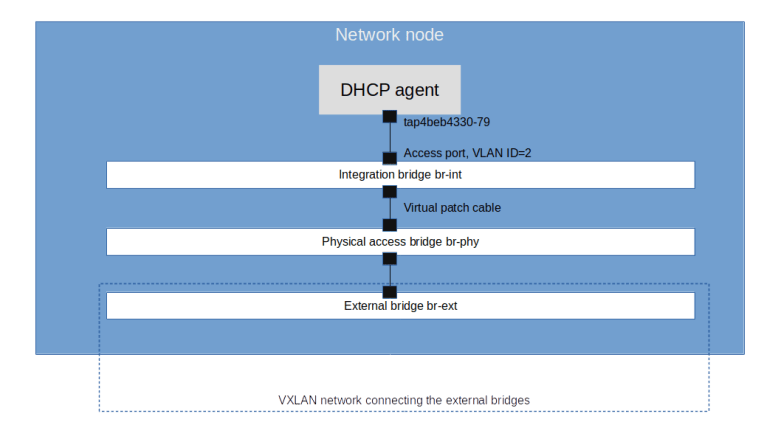
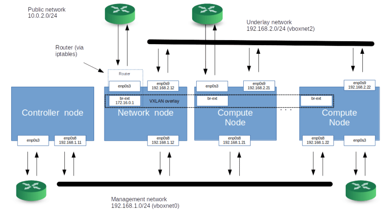
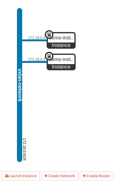
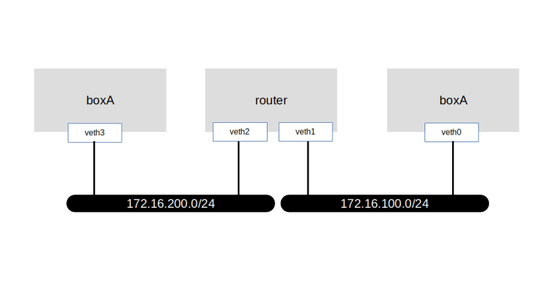
Let us now try to understand how the metadata service of OpenStack works. To do this, let us run an example configuration (we will use the configuration of Lab 10) and SSH into one of the demo instances in our VXLAN network (this is an important detail, the behavior for instances on the flat network is different, see below).

git clone https://github.com/christianb93/openstack-labs
cd openstack-labs/Lab10
vagrant up 
ansible-playbook -i hosts.ini site.yaml
ansible-playbook -i hosts.ini demo.yaml
vagrant ssh network
source demo-openrc
openstack server ssh \
   --identity demo-key  \
   --public \
   --login cirros \
   demo-instance-1
curl http://169.254.169.254/1.0/meta-data

This should give you an output very similar to the one that you have seen on EC2, and in fact, OpenStack implements the EC2 metadata protocol (it also implements its own protocol, more on this in a later section).

At this point, we could just accept that this works, be happy and relax, but if you have followed my posts, you will know that simply accepting that it works is not the idea of this blog – why does it work?

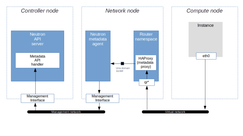
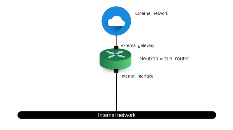
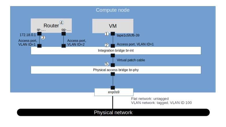
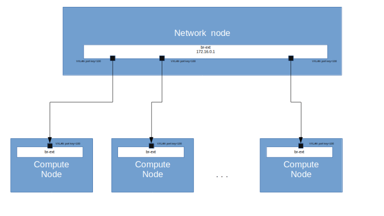
The first thing that comes to ones mind when trying to understand how this request leaves the instance and where it is answered is to check the routing on the instance by running route -n. We find that there is in fact a static route to the IP address 160.254.169.254 which points to the gateway address 172.18.0.1, i.e. to our virtual router. In fact, this route is provided by the DHCP service, as you will easily be able to confirm when you have read my recent post on this topic.

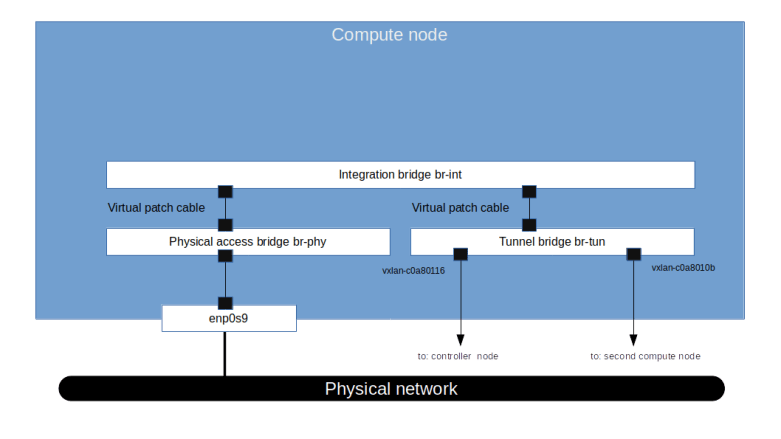
So the request goes to the router. We know that in OpenStack, a router is realized as a namespace on the node on which the L3 agent is running, i.e. on the network node in our case. Let us now peep inside this namespace and try to see which processes are running within it and how its network is configured. Back on the network node, run

router_id=$(openstack router show \
  demo-router  \
  -f value\
   -c id)
ns_id="qrouter-$router_id"
sudo ip netns exec $ns_id  iptables -S -t nat
pid=$(sudo ip netns pid $ns_id)
ps fw -p $pid 

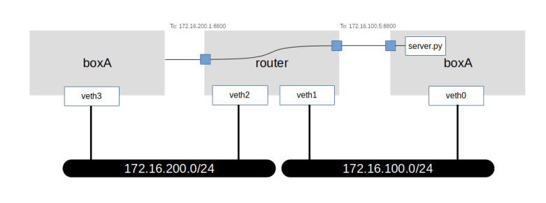
From the output, we learn two things. First, we find that in the router namespace, there is an iptables rule that redirects traffic targeted towards the IP address 169.254.169.254:80 to port 9697 on the local machine. Second, there is an instance of the HAProxy reverse proxy running in this namespace. The command line with which this proxy was started points us to its configuration file, which in turn will tell us that the HAProxy is listening on exactly this port and redirecting the request to a Unix domain socket /var/lib/neutron/metadata_proxy.

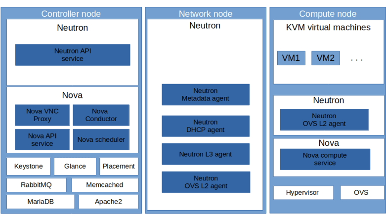
If we use sudo netstat -a -p to find out who is listening on this socket, we will see that the socket is owned by an instance of the Neutron metadata agent which essentially forwards the request.

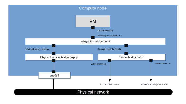
The IP address and port to which the request is forwarded are taken from the configuration file /etc/neutron/metadata_agent.ini of the Neutron metadata agent. When we look up these values, we find, however, that the (default) port 8775 is not the usual API endpoint of the Nova server. which is listening in port 8774. So the request is not yet going to the API. Instead, port 8775 is used by the Nova metadata API handler, which is technically a part of the Nova API server. This service will accept the incoming request, retrieve the instance and its metadata from the database and send the reply, which then goes all the way back to the instance. Thus the following picture emerges from our discussion.

NeutronNovaMetadataServer

Now clearly there is a part of the story that we have not yet discussed, as some points are still a bit mysterious. How, for instance, does the Nova API server know for which instance the metadata is requested? And how is the request authorized without a Keystone token?

To answer these questions, it is useful to dump a request across the chain using tcpdump sessions on the router interface and the management interface on the controller. For the first session, SSH into the network node and run

source demo-openrc
router_id=$(openstack router show \
  demo-router  \
  -f value\
   -c id)
ns_id="qrouter-$router_id"
interface_id=$(sudo ip netns exec \
  $ns_id tcpdump -D \
  | grep "qr" | awk -F "." '{print $1}')
sudo ip netns \
  exec $ns_id tcpdump \
  -i $interface_id \
  -e -vv port not 22

Then, open a second terminal and SSH into the controller node. On the controller node, start a tcpdump session on the management interface to listen for traffic targeted to the port 8775.

sudo tcpdump -i enp0s8 -e -vv -A port 8775

Finally, connect to the instance demo-instance-1 using SSH, run

curl http://169.254.169.254/1.0/meta-data

and enjoy the output of the tcpdump processes. When you read this output, you will see the original GET request showing up on the router interface. On the interface of the controller, however, you will see that the Neutron agent has added some headers to the request. Specifically, we see the following headers.

  • X-Forwarded-For contains the IP address of the instance that made the request and is added to the request by the HAProxy
  • X-Instance-ID contains the UUID of the instance and is determined by the Neutron agent by looking up the port to which the IP address belongs
  • X-Tenant-ID contains the ID of the project to which the instance belongs
  • X-Instance-ID-Signature contains a signature of the instance ID

The instance ID and the project ID in the header are used by the Nova metadata handler to look up the instance in the database and to verify that the instance really belongs to the project in the request header. The signature of the instance ID is used to authorize the request. In fact, the Neutron metadata agent uses a shared secret that is contained in the configuration of the agent and the Nova server as (metadata_proxy_shared_secret) to sign the instance ID (using the HMAC signature specified in RFC 2104) and the Nova server uses the same secret to verify the signature. If this verification fails, the request is rejected. This mechanism replaces the usual token based authorization method used for the main Nova API.

Metadata requests on isolated networks

We can now understand how the metadata request is served. The request leaves the instance via the virtual network, reaches the router, is picked up by the HAProxy, forwarded to the agent and … but wait .. what if there is no router on the network?

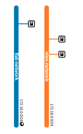
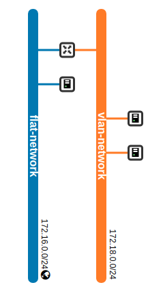
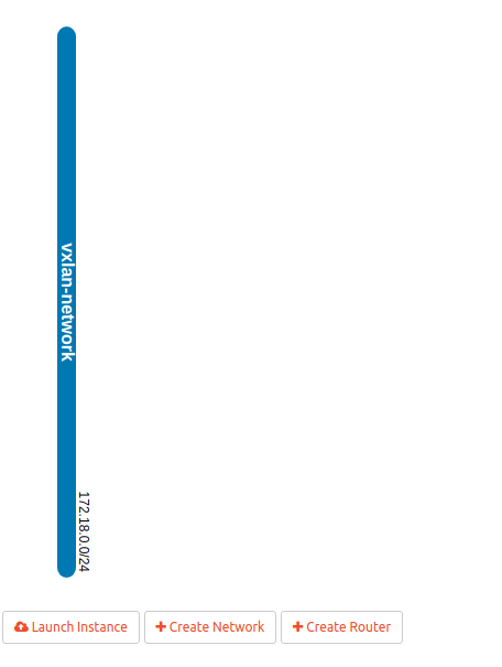
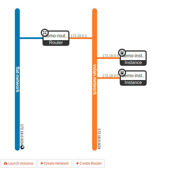
Recall that in our test configuration, there are two virtual networks, one flat network (which is connected to the external bridge br-ext on each compute node and the network node) and one VXLAN network.

DedicatedNetworkNodeVirtualTopology

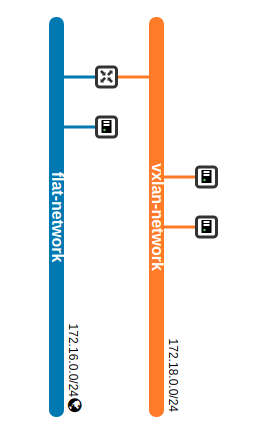
So far, we have been submitting metadata requests from an instance connected to the VXLAN network. On this network, a router exists and serves as a gateway, so the mechanism outlined above works. In the flat network, however, the gateway is an external (from the point of view of Neutron) router and cannot handle metadata requests for us.

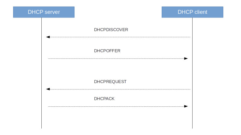
To solve this issue, Neutron has the ability to let the DHCP server forward metadata requests. This option is activated with the flag enable_isolated_metadata in the configuration of the DHCP agent. When this flag is set and the agent detects that it is running in an isolated network (i.e. a network whose gateways is not a Neutron provided virtual router), it will do two things. First, it will, as part of a DHCPOFFER message, use the DHCP option 121 to ask the client to set a static route to 169.254.169.254 pointing to its own IP address. Then, it will spawn an instance of HAProxy in its own namespace and add the IP address 169.254.169.254 as second IP address to its own interface (I will not go into the detailed analysis to verify these claims, but if you have followed this post up to this point and read my last post on Neutron DHCP server, you should be able to run the diagnosis to see this yourself). The HAProxy will then again use a Unix domain socket to forward the request to the Neutron metadata agent.

NeutronNovaMetadataServerIsolated

We could even ask the DHCP agent to provide metadata services for all networks by setting the flag force_metadata to true in the configuration of the DHCP agent.

The OpenStack metadata protocol

So far we have made our sample metadata requests using the EC2 protocol. In addition to this protocol, the Nova Metadata handler is also able to serve requests that use the OpenStack specific protocol which is available under the URL http://169.254.169.254/openstack/latest. This offers you several data structures, one of them being the entire instance metadata as a JSON structure. To test this, SSH into an arbitrary test instance and run

curl http://169.254.169.254/openstack/latest/meta_data.json

Here is a redacted version of the output, piped through jq to increase readability.

{
  "uuid": "74e3dc71-1acc-4a38-82dc-a268cf5f8f41",
  "public_keys": {
    "demo-key": "ssh-rsa REDACTED"
  },
  "keys": [
    {
      "name": "demo-key",
      "type": "ssh",
      "data": "ssh-rsa REDACTED"
    }
  ],
  "hostname": "demo-instance-3.novalocal",
  "name": "demo-instance-3",
  "launch_index": 0,
  "availability_zone": "nova",
  "random_seed": "IS3w...",
  "project_id": "5ce6e231b4cd483f9c35cd6f90ba5fa8",
  "devices": []
}

We see that the data includes the SSH keys associated with the instance, the hostname, availability zone and the ID of the project to which the instance belongs. Another interesting structure is obtained if we replace meta_data.json by network_data.json

{
  "links": [
    {
      "id": "tapb21a530c-59",
      "vif_id": "b21a530c-599c-4275-bda2-6644cf55ed23",
      "type": "ovs",
      "mtu": 1450,
      "ethernet_mac_address": "fa:16:3e:c0:a9:89"
    }
  ],
  "networks": [
    {
      "id": "network0",
      "type": "ipv4_dhcp",
      "link": "tapb21a530c-59",
      "network_id": "78440978-9f8f-4c59-a254-99289dad3c81"
    }
  ],
  "services": []
}

We see that we get a list of network interfaces and networks attached to the machine, which contains useful information like the MAC addresses, the MTU and even the interface type (OVS internal device in our case).

Working with user data

So far we have discussed instance metadata, i.e. data provided by OpenStack. In addition, like most other cloud platforms, OpenStack allows you to attach user data to an instance, i.e. user defined data which can then be retrieved from inside the instance using exactly the same way. To see this in action, let us first delete our demo instance and re-create it (OpenStack allows you to specify user data at instance creation time). Log into the network node and run the following commands.

source demo-openrc
echo "test" > test.data
openstack server delete demo-instance-3
openstack server create \
   --network flat-network \
   --key demo-key \
   --image cirros \
   --flavor m1.nano \
   --user-data test.data demo-instance-3 
status=""
until [ "$status" == "ACTIVE" ]; do
  status=$(openstack server show \
    demo-instance-3  \
    -f shell \
    | awk -F "=" '/status/ { print $2}' \
    | sed s/\"//g)
  sleep 3
done
sleep 3
openstack server ssh \
   --login cirros\
   --private \
   --option StrictHostKeyChecking=no \
   --identity demo-key demo-instance-3

Here we first create a file with some test content. Then, we delete the server demo-instance-3 and re-create it, this time passing the file that we have just created as user data. We then wait until the instance is active, wait for a few seconds to allow the SSH daemon in the instance to come up, and then SSH into the server. When you now run

curl 169.254.169.254/1.0/user-data

inside the instance, you should see the contents of the file test.data.

This is nice, but to be really useful, we need some process in the instance which reads and processes the user data. Enter cloud-init. As already mentioned above, the cirros image that we have used so far does not contain cloud-init. So to play with it, download and install the Ubuntu cloud image as described in my earlier post on Glance. As the size of the image exceeds the resources of the flavor that we have used so far, we also have to create a new flavor as admin user.

source admin-openrc
openstack flavor create \
  --disk 5 \
  --ram 1024 \
  --vcpus 1 m1.tiny

Next, we will create a file holding the user data in a format that cloud-init is able to process. This could be a file starting with

#!/bin/bash

to indicate that this is a shell script that should be run via bash, or a cloud-init configuration file starting with

#cloud-config

Let us try the latter. Using the editor of your choice, create a file called cloud-init-config on the network node with the following content which will instruct cloud-init to create a file called /tmp/foo with content bar.

#cloud-config
write_files:
-   content: bar
    path: /tmp/foo
    permissions: '0644'

Note the indentation – this needs to be valid YAML syntax. Once done, let us recreate our instance using the new image.

source demo-openrc
openstack server delete demo-instance-3
openstack server create \
   --network flat-network \
   --key demo-key \
   --image ubuntu-bionic \
   --flavor m1.tiny \
   --user-data cloud-init-config demo-instance-3 
status=""
until [ "$status" == "ACTIVE" ]; do
  status=$(openstack server show \
    demo-instance-3  \
    -f shell \
    | awk -F "=" '/status/ { print $2}' \
    | sed s/\"//g)
  sleep 3
done
sleep 120
openstack server ssh \
   --login ubuntu\
   --private \
   --option StrictHostKeyChecking=no \
   --identity demo-key demo-instance-3

When using this image in our environment with nested virtualization, it can take as long as one or two minutes until the SSH daemon is ready and we can log into our instance. When you are logged in, you should see a new file /tmp/foo which contains the string bar, as expected.

Of course this is still a trivial example, and there is much more that you can do with cloud-init: creating new users (be careful, this will overwrite the standard user – add the default user to avoid this), installing packages, running arbitrary scripts, configuring the network and so forth. But this is a post on the metadata mechanism provided by OpenStack, and not on cloud-init, so we will leave that topic for now.

This post also concludes – at least for the time being – our series focussing on Neutron. We will now turn to block storage – how block storage is provisioned and used on the OpenStack platform, how Cinder is installed and works under the hood and how all this relates to standards like iSCSI and the Linux logical volume manager LVM.

OpenStack Neutron – DHCP and DNS

In a cloud environment, a virtual instance typically uses a DHCP server to receive its assigned IP address and DNS services to resolve IP addresses. In this post, we will look at how these services are realized in our OpenStack playground environment.

DHCP basics

To understand what follows, it is helpful to quickly recap the basis mechanisms behind the DHCP protocol. Historically, the DHCP protocol originated from the earlier BOOTP protocol, which was developed by Sun Microsystems (my first employer, back in the good old days, sigh…) to support diskless workstations which, at boot time, need to retrieve their network configuration, the name of a kernel image (which could subsequently be retrieved using TFTP) and an NFS share to be used for the root partition. The DHCP protocol builds on the BOOTP standard and extends BOOTP, for instance by adding the ability to deliver more configuration options than BOOTP is capable of.

DHCP is a client-server protocol using UDP with the standardized ports 67 (server) and 68 (client). At boot time, a client sends a DHCPDISCOVER message to request configuration data. In reply, the server sends a DHCPOFFER message to the client, offering configuration data including an IP address. More than one server can answer a discovery message, and thus a client might receive more than one offer. The DCHCP client then sends a DHCPREQUEST to all servers, containing the ID of an offer that the client wishes to accept. The server from which that offer originates then replies with a DHCPACK to complete the handshake, all other servers simply record the fact that the IP address that they have offered is again available. Finally, a DHCP client can release an IP address again sending the DHCPRELEASE message.

There are a few additional message types like DHCPINFORM which a client can use to only request configuration parameters if it already has an IP address, or a DHCPDECLINE message that a client sends to a server if it determines (using ARP) that a message offered by the server is already in use, but these message types do usually not take part in a standard bootstrap sequence which is summarized in the diagram below.

DHCPBootstrap

We have said that DHCP is using UDP which again is sitting on top of the IP protocol. This raises an interesting chicken-egg problem – how can a client use DHCP to talk to a server if is does not yet have an IP address?

The answer is of course to use broadcasts. Initially, a client sends a DHCP request to the IP broadcast address 255.255.255.255 and the Ethernet broadcast address ff:ff:ff:ff:ff:ff. The IP source address of this request is 0.0.0.0.

Then, the server responds with a DHCPOFFER directed towards the MAC address of the client and using the offered IP address as IP target address. The DHCPREQUEST is again a broadcast (this is required as it needs to go to all DHCP servers on the subnet), and the acknowledge message is again a unicast packet.

This process assumes that the client is able to receive an IP message directed to an IP address which is not (yet) the IP address of one of its interfaces. As most Unix-like operating systems (including Linux) do not allow this, DHCP clients typically use a raw socket to receive all incoming IP traffic (see for instance the relevant code of the udhcp client which is part of BusyBox which uses a so-called packet socket initially and only switches to an ordinary socket once the interface is fully configured). Alternatively, there is a flag that a client can set to indicate that it cannot deal with unicast packets before the interface is fully configured, in which case the server will also use broadcasting for its reply messages.

Note that, as specified in RFC 922, a router will not forward IP broadcasts directed to the broadcast address 255.255.255.255. Therefore, without further precautions, a DHCP exchange cannot pass a router, which implies that a DHCP server must be present on every subnet. It is, however, possible to run a so-called DHCP relay which forwards DHCP requests to a DHCP server in a different network. Neutron will, by default, start a DHCP server for each individual virtual network (unless DHCP is disabled for all subnets in the network).

One of the reasons why the DHCP protocol is more powerful than the older BOOTP protocol is that the DHCP protocol is designed to provide a basically unlimited number of configuration items to a client using so-called DHCP options. The allowed options are defined in various RFCs (see this page for an overview maintained by the IANA organisation). A few notable options which are relevant for us are

  • Option 1: subnet mask, used to inform the client about the subnet in which the provided IP address is valid
  • Option 3: list of routers, where the first router is typically used as gateway by the client
  • Option 6: DNS server to use
  • Option 28: broadcast address for the clients subnet
  • Option 121: classless static routes (replaces the older option 33) that are transmitted from the server to the client and supposed to be added to the routing table by the client

DHCP implementation in OpenStack

After this general introduction, let us now try to understand how all this is implemented in OpenStack. To be able to play around and observe the system behavior, let us bring up the configuration of Lab 10 once more.

git clone https://github.com/christianb93/openstack-labs
cd openstack-labs/Lab10
vagrant up
ansible-playbook -i hosts.ini site.yaml
ansible-playbook -i hosts.ini demo.yaml

This will install OpenStack with a separate network node, create two networks and bring up instances on each of these networks.

Now, for each virtual network, Neutron will create a network namespace on the network node (or, more precisely, on the node on which the DHCP agent is running) and spawn a separate DHCP server process in each of these namespaces. To verify this, run

sudo ip netns list

on the network node. You should see three namespaces, two of them starting with “qdhcp-“, followed by the ID of one of the two networks that we have created. Let us focus our investigation on the flat network, and figure out which processes this namespace contains. The following sequence of commands will determine the network ID, derive the name of the namespace and list all processes running in this namespace.

source demo-openrc
network_id=$(openstack network show \
    flat-network \
    -f yaml | egrep "^id: " | awk '{ print $2}')
ns_id="qdhcp-$network_id"
pids=$(sudo ip netns pid $ns_id)
for pid in $pids; do
  ps --no-headers -f --pid $pid
done

We see that there are two processes running inside the namespace – an instance of the lightweight DHCP server and DNS forwarder dnsmasq and a HA proxy process (which handles metadata requests, more on this in a separate post). It is interesting to look at the full command line which has been used to start the dnsmasq process. Among the long list of options, you will find two options that are especially relevant.

First, the process is started using the --no-hosts flag. Usually, dnsmasq will read the content of the local /etc/hosts file and return the name resolutions defined there. Here, this is disabled, as otherwise an instance could retrieve the IP addresses of the OpenStack nodes. The process is also started with –no-resolv to skip reading of the local resolver configuration on the network node.

Second, the dnsmasq instance is started with the --dhcp-host-file option, which, in combination with the static keyword in the --dhcp-range option, restricts the address allocations that the DHCP server will hand out to those defined in the provided file. This file is maintained by the DHCP agent process. Thus the DHCP server will not actually perform address allocations, but is only a way to communicate the address allocations that Neutron has already prepared to a client.

To better understand how this actually works, let us go through the process of starting a virtual machine and allocating an IP address in a bit more detail. Here is a summary of what happens.

IPAddressAllocation

First, when a user requests the creation of a virtual machine, Nova will ask Neutron to create a port (1). This request will eventually hit the create_port method of the ML2 plugin. The plugin will then create the port as a database object and, in the course of doing this, reach out to the configured IPAM driver to obtain an IP address for this port.

Once the port has been created, an RPC message is sent to the DHCP agent (2). The agent will then invoke the responsible DHCP driver (which in our case is the Linux DHCP driver) to re-build the hosts file and send a SIGHUP signal to the actual dnsmasq process in order to reload the changed file (5)

At some later point in the provisioning process, the Nova compute agent will create the VM (6) which will start its boot process. As part of the boot process, a DHCP discover broadcast will be sent out to the network (7). The dnsmasq process will pick up this request, consult the hosts file, read the pre-determined IP address and send a corresponding DHCP offer to the VM. The VM will usually accept this offer and configure its network interface accordingly.

Network setup

We have now understood how the DHCP server handles address allocations. Let us now try to figure out how the DHCP server is attached to the virtual network which it server.

To examine the setup, log into the network node again and repeat the above commands to again populate the environment variable ns_id with the ID of the namespace in which the DHCP server is running. Then, run the following commands to gather information on the network setup within the namespace.

sudo ip netns exec $ns_id ip link show

We see that apart from the loopback device, the DHCP namespace has one device with a name composed of the fixed part tap followed by a unique identifier (the first few characters of the ID of the corresponding port). When you run sudo ovs-vsctl show on the network node, you will see that this device (which is actually an OVS created device) is attached to the integration bridge br-int as an access port. When you dump the OpenFlow rules on the integration bridge and the physical bridge, you will see that for packets with this VLAN ID, the VLAN tag is stripped off at the physical bridge and the packet eventually reaches the external bridge br-ext, confirming that the DHCP agent is actually connected to the flat network that we have created (based on our VXLAN network that we have built outside of OpenStack).

DHCPAgentNetworkSetup

Also note that in our case, the interface used by the DHCP server has actually two IP addresses assigned, one being the second IP address on the subnet (172.16.0.2), and the second one being the address of the metadata server (which might seem a bit strange, but again this will be the topic of the next post).

If you want to see the DHCP protocol in action, you can install dhcpdump on the network node, attach to the network namespace and run a dump on the interface while bringing up an instance on the network. Here is a sequence of commands that will start a dump.

source admin-openrc
sudo apt-get install dhcpdump
port_id=$(openstack port list \
  --device-owner network:dhcp \
  --network flat-network \
  -f value | awk '{ print $1}')
interface="tap$port_id"
interface=${interface:0:14}
source demo-openrc
network_id=$(openstack network show \
    flat-network \
    -f yaml | egrep "^id: " | awk '{ print $2}')
ns_id="qdhcp-$network_id"
sudo ip netns exec $ns_id dhcpdump -i $interface

In a separate window (either on the network node or any other node), enter the following commands to bring up an additional instance

source demo-openrc
openstack server create \
  --flavor m1.nano \
  --network flat-network \
  --key demo-key \
  --image cirros demo-instance-4

You should now see the sequence of DHCP messages displayed in the diagram above, starting with the DHCPDISCOVER sent by the newly created machine and completed by the DHCPACK.

Configuration of the DHCP agent

Let us now go through some of the configuration options that we have for the DHCP agent in the file /etc/neutron/dhcp_agent.ini. First, there is the interface_driver which we have set to openvswitch. This is the driver that the DHCP agent will use to set up and wire up the interface in the DHCP server namespace. Then, there is the dhcp_driver which points to the driver class used by the DHCP agent to control the DHCP server process (dnsmasq).

Let us also discuss a few options which are relevant for the name resolution process. Recall that dnsmasq is not only a DHCP server, but can also act as DNS forwarder, and these settings control this functionality.

  • We have seen above that the dnsmasq process is started with the –no-resolv option in order to skip the evaluation of the /etc/resolv.conf file on the network node. If we set the configuration option dnsmasq_local_resolv to true, then dnsmasq will read this configuration and effectively be able to use the DNS configuration of the network node to provide DNS services to instances.
  • A similar settting is dnsmasq_dns_servers. This configuration item can be used to provide a list of DNS servers to which dnsmasq will forward name resolution requests

DNS configuration options for OpenStack

The configuration items above give us a few options that we have to control the DNS resolution offered to the instances.

First, we can set dnsmasq_local_resolv to true. When you do this and restart the DHCP agent, all dnsmasq processes will be restarted without the –no-resolv option. The DHCP server will then instruct instances to use its own IP address as the address of a DNS server, and will leverage the resolver configuration on the network node to forward requests. Note, however, that this will only work if the nameserver in /etc/resolv.conf on the network node is set to a server which can be reached from within the DHCP namespace, which will typically not be the case (on a typical Ubuntu system, name resolution is done using systemd-resolved which will listen on a loopback interface on the network node which cannot be reached from within that namespace).

The second option that we have is to put one or more DNS servers which are reachable from the virtual network into the configuration item dnsmasq_dns_servers. This will instruct the DHCP agent to start the dnsmasq processes with the –server flag, thus specifying a name server to which dnsmasq is supposed to forward requests. Assuming that this server is reachable from the network namespace in which dnsmasq is running (i.e. from the virtual network to which the DHCP server is attached), this will provide name resolution services using this nameserver for all instances on this network.

As the configuration file of the DHCP agent is applied for all networks, using this option implies that all instances will be using this DNS server, regardless of the network to which they are attached. In more complex settings, this is sometimes not possible. For these situations, Neutron offers a third option to configure DNS resolution – defining a DNS server per subnet. In fact, a list of DNS servers is an attribute of each subnet. To set the DNS server 8.8.8.8 for our flat subnet, use

source admin-openrc 
openstack subnet set \
  --dns-nameserver 8.8.8.8 flat-subnet
source demo-openrc

When you now restart the DHCP agent, you will see that the DHCP agent has added a line to the options file for the dnsmasq process which sets the DNS server for this specific subnet to 8.8.8.8.

Note that this third option works differently from the first two options in that it really sets the DNS server in the instances. In fact, this option does not govern the resolution process when using dnsmasq as a nameserver, but determines the nameserver that will be provided to the instances at boot time via DHCP, so that the instances will directly contact this nameserver. Our first two configuration did work differently, as in both options, the nameserver known to the instance will be the DHCP server, and the DHCP server will then forward the request to the configured name server. The diagram below summarizes this mechanism.

DNSConfigurationOptions

Of course you can combine these settings – use dnsmasq_dns_servers to enable the dnsmasq process to serve and forward DNS requests, and, if needed, override this using a subnet specific DNS server for individual subnets.

This completes our investigation of DHCP and DNS handling on OpenStack. In the next post, we will turn to a topic that we have already touched upon several times – instance metadata.


OpenStack Neutron – building virtual routers

In a previous post, we have set up an environment with a flat network (connected to the outside world, in this case to our lab host). In a typical environment, such a network is combined with several internal virtual networks, connected by a router. Today, we will see how an OpenStack router can be used to realize such a setup.

Installing and setting up the L3 agent

OpenStack offers different models to operate a virtual router. The model that we discuss in this post is sometimes called a “legacy router”, and is realized by a router running on one of the controller hosts, which implies that the routing functionality is no longer available when this host goes down. In addition, Neutron offers more advanced models like a distributed virtual router (DVR), but this is beyond the scope of todays post.

To make the routing functionality available, we have to install respectively enable two additional pieces of software:

  • The Routing API is provided by an extension which needs to be loaded by the Neutron server upon startup. To achieve this, this extension needs to be added to the service_plugins list in the Neutron configuration file neutron.conf
  • The routing functionality itself is provided by an agent, the L3 agent, which needs to be installed on the controller node

In addition to installing these two components, there are a few changes to the configuration we need to make. First, of course, the L3 agent comes with its own configuration file that we need to adapt. Specifically, there are two changes that we make for this lab. First, we set the interface driver to openvswitch, and second, we ask the L3 agent not to provide a route to the metadata proxy by setting enable_metadata_proxy to false, as we use the mechanism provided by the DHCP agent.

In addition, we change the configuration of the Horizon dashboard to make the L3 functionality available in the GUI as well (this is done by setting the flag horizon_enable_router in the configuration to “True”).

All this can again be done in our lab environment by running the scripts for Lab 8. In addition, we run the demo playbook which will set up a VLAN network with VLAN ID 100 and two instances attached to it (demo-instance-1 and demo-instance 3) and a flat, external network with one instance (demo-instance-3).

git clone https://github.com/christianb93/openstack-labs
cd Lab8
vagrant up
ansible-playbook -i hosts.ini site.yaml
ansible-playbook -i hosts.ini demo.yaml

Setting up our first router

Before setting up our first router, let us inspect the network topology that we have created. The Horizon dashboard has a nice graphical representation of the network topology.

Networks

We see that we have two virtual Ethernet networks, carrying one IP network each. The network on the left – marked as external – is the flat network, with an IP subnet with CIDR 172.18.0.0/24. The network on the right is the VLAN network, with IP range 172.16.0.0./24.

Now let us create and set up the router. This happens in several steps. First, we create the router itself. This is done using the credentials of the demo user, so that the router will be part of the demo project.

vagrant ssh controller
source demo-openrc
openstack router create demo-router

At this point, the router exists as an object, and there is an entry for it in the Neutron database (table routers). However, the router is not yet connected to any network. Let us do this next.

It is important to understand that, similar to a physical router, a Neutron virtual router has two interfaces connected to two different networks, and, again as in the physical network world, the setup is not symmetric. Instead, there is one network which is considered external and one internal network. By default, the router will allow for traffic from the internal network to the external network, but will not allow any incoming connections from the external network into the internal networks, very similar to the cable modem that you might have at home to connect to this WordPress site.

NeutronRouter

Correspondingly, the way how the external network and the internal network are attached to the router differ. Let us start with the external network. The connection to the external network is called the external gateway of the router and can be assigned using the set command on the router.

openstack router set \
   --external-gateway=flat-network\
   demo-router

When you run this command and inspect the database once more, you will see that the column gw_port_id has been populated. In addition, listing the ports will demonstrate that OpenStack has created a port which is attached to the router (this port is visible in the database but not via the CLI as the demo user, as the port is not owned by this user) and has received an IP address on the external network.

To complete the setup of the router, we now have to connect the router to an internal network. Note that this needs to be done by the administrator, so we first have to source the credentials of the admin user.

source admin-openrc
openstack router add subnet demo-router vlan-subnet

When we now log into the Horizon GUI as the demo user and ask Horizon to display the network topology, we get the following result.

NetworkWithRouter

We can reach the flat network (and the lab host) from the internal network, but not the other way around. You can verify this by logging into demo-instance-1 via the Horizon VNC console and trying to ping demo-instance-3.

Now let us try to understand how the router actually works. Of course, somewhere behind the scenes, Linux routing mechanisms and iptables are used. One could try to implement a router by manipulating the network stack on the controller node, but this would be difficult as the configuration for different routers might conflict. To avoid this, Neutron creates a dedicated network namespace for each router on the node on which the L3 agent is running.

The name of this namespace is qrouter-, followed by the ID of the virtual router (here “q” stands for “Quantum” which was the name of what is now known as Neutron some years ago). To analyze the network stack within this namespace, let us retrieve its ID and spawn a shell inside the namespace.

netns=$(ip netns list \
        | grep "qrouter" \
        | awk '{print $1'})
sudo ip netns exec $netns /bin/bash

Running ifconfig -a and route -n shows that, as expected, the router has two virtual interfaces (both created by OVS). One interface starting with “qg” is the external gateway, the second one starting with “qr” is connected to the internal network. There are two routes defined, corresponding to the two subnets to which the respective interfaces are assigned.

Let us now inspect the iptables configuration. Running iptables -S -t nat reveals that Neutron has added an SNAT (source network address translation) rule that applies to traffic coming from the internal interface. This rule will replace the source IP address of the outgoing traffic by the IP address of the router on the external network.

To understand how the router is attached to the virtual network infrastructure, leave the namespace again and display the bridge configuration using sudo ovs-vsctl show. This will show you that the two router interfaces are both attached to the integration bridge.

NeutronRouterEgress

Let us now see how traffic from a VM on the internal network flows through the stack. Suppose an application inside the VM tries to reach the external network. As inside the VM, the default route goes to 172.18.0.1, the routing mechanism inside the VM targets the packet towards the qr-interface of the router. The packet leaves the VM through the tap interface (1). The packet enters the bridge via the access port and receives a local VLAN tag (2), then travels across the bridge to the port to which the qr-interface is attached. This port is an access port with the same local VLAN tag as the virtual machine, so it leaves the bridge as untagged traffic and enters the router (3).

Within the router, SNAT takes place (4) and the packet is forwarded to the qg-interface. This interface is attached to the integration bridge as access port with local VLAN ID 2. The packet then travels to the physical bridge (5), where the VLAN tag is stripped off and the packet hits the physical networks as part of the native network corresponding to the flat network.

As the IP source address is the address of the router on the external network, the response will be directed towards the qg-interface. It will enter the integration bridge coming from the physical bridge as untagged traffic, receive local VLAN ID 2 and end up at the qg-access port. The packet then flows back through the router, is leaving it again at the qr interface, appears with local VLAN tag 1 on the integration bridge and eventually reaches the VM.

There is one more detail that deserves being mentioned. When you inspect the iptables rules in the mangle table of the router namespace, you will see some rules that add marks to incoming packets, which are later evaluated in the nat and filter tables. These marks are used to implement a feature called address scopes. Essentially, address scopes are reflecting routing domains in OpenStack, the idea being that two networks that belong to the same address scope are supposed to have compatible, non-overlapping IP address ranges so that no NATing is needed when crossing the boundary between these two networks, while a direct connection between two different address scopes should not be possible.

Floating IPs

So far, we have set up a router which performs a classical SNAT to allow traffic from the internal network to appear on the external network as if it came from the router. To be able to establish a connection from the external network into the internal network, however, we need more.

In a physical infrastructure, you would use DNAT (destination netting) to achieve this. In OpenStack, this is realized via a floating IP. This is an IP address on the external network for which DNAT will be performed to pass traffic targeted to this IP address to a VM on the internal network.

To see how this works, let us first create a floating IP, store the ID of the floating IP that we create in a variable and display the details of the floating IP.

source demo-openrc
out=$(openstack floating ip create \
         -f shell \
         --subnet flat-subnet\
           flat-network)
floatingIP=$(eval $out ; echo $id)
openstack floating ip show $floatingIP

When you display the details of the floating IP, you will see that Neutron has assigned an IP from the external network (the flat network), more precisely from the network and subnet that we have specified during creation.

This floating IP is still fully “floating”, i.e. not yet attached to any actual instance. Let us now retrieve the port of the server demo-instance-1 and attach the floating IP to this port.

port=$(openstack port list \
         --server demo-instance-1 \
         -f value \
         | awk {'print $1}')
openstack floating ip set --port $port $floatingIP

When we now display the floating IP again, we see that floating IP is now associated with the fixed IP address of the instance demo-instance-1.

Now leave the controller node again. Back on the lab host, you should now be able to ping the floating IP (using the IP on the external network, i.e. from the 172.16.0.0/24 network) and to use it to SSH into the instance.

Let us now try to understand how the configuration of the router has changed. For that purpose, enter the namespace again as above and run ip addr. This will show you that now, the external gateway interface (the qg interface) has now two IP addresses on the external network – the IP address of the router and the floating IP. Thus, this interface will respond to ARP requests for the floating IP with its MAC address. When we now inspect the NAT tables again, we see that there are two new rules. First, there is an additional source NAT rule which replaces the source IP address by the floating IP for traffic coming from the VM. Second, there is now – as expected – a destination NAT rule. This rule applies to traffic directed to the floating IP and replaces the target address with the VM IP address, i.e. with the corresponding fixed IP on the internal network.

We can now understand how a ping from the lab host to the floating IP flows through the stack. On the lab host, the packet is routed to the vboxnet1 interface and shows up at enp0s9 on the controller node. From there, it travels through the physical bridge up to the integration bridge and into the router. There, the DNAT processing takes place, and the target IP address is replaced by that of the VM. The packet leaves the router at the internal qr-interface, travels across the integration bridge and eventually reaches the VM.

Direct access to the internal network

We have seen that in order to connect to our VMs using SSH, we first need to build a router to establish connectivity and assign a floating IP address. Things can go wrong, and if that operation fails for whatever reason or the machines are still not reachable, you might want to find a different way to get access to the instances. Of course there is the noVNC client built into Horizon, but it is more convenient to get a direct SSH connection without relying on the router. Here is an approach how this can be done.

Recall that on the physical bridge on the controller node, the internal network has the VLAN segmentation ID 100. Thus to access the VM (or any other port on the internal network), we need to tag our traffic with the VLAN tag 100 and direct it towards the bridge.

The easiest way to do this is to add another access port to the physical bridge, to assign an IP address to it which is part of the subnet on the internal network and to establish a route to the internal network from this device.

vagrant ssh controller
sudo ovs-vsctl add-port br-phys vlan100 tag=100 \
     -- set interface vlan100 type=internal 
sudo ip addr add 172.18.0.100/24 dev vlan100
sudo ip link set vlan100 up

Now you should to be able to ping any instance on the internal VLAN network and SSH into it as usual from the controller node.

Why does this work? The upshot of our discussion above is that the interaction of local VLAN tagging, global VLAN tagging and the integration bridge flow rules effectively attach all virtual machines in our internal network via access ports with tagging 100 to the physical network infrastructure, so that they all communicate via VLAN 100. What we have done is to simply create another network device called vlan100 which is also connected to this VLAN. Therefore, it is effectively on one Ethernet segment with our first two demo instances. We can therefore assign an IP address to it and then use it to reach these instances. Essentially, this adds an interface to the controller which is connected to the virtual VLAN network so that we can reach each port on this network from the controller node (be it on the controller node or a compute node).

There is much more we could say about routers in OpenStack, but we leave that topic for the time being and move on to the next post, in which we will discuss overlay networks using VXLAN.

OpenStack Neutron – running Neutron with a separate network node

So far, our OpenStack control plane setup was rather simple – we had a couple of compute nodes, and all other services were running on the same controller node. In practice, this does not only create a single point of failure, but also a fairly high traffic on the network interfaces. In this post, we will move towards a more distributed setup with a dedicated network node.

OpenStack nodes and their roles

Before we plan our new topology, let us quickly try to understand what nodes we have used so far. Recall that each node has an Ansible hostname which is the name returned by the Ansible variable inventory_hostname and defined in the inventory file. In addition, each node has a DNS name, and during our installation procedure, we adapt the /etc/hosts file on each node so that DNS names and Ansible hostnames are identical. A host called, for instance, controller in the Ansible inventory will therefore be reachable under this name across the cluster.

The following table lists the types of nodes (defined by the services running on them) and the Ansible hostnames used so far.

Node type Description Hostname
api_node Node on which all APIs are exposed. This will typically be the controller node, but could also be a load balancer in a HA setup controller
db_node Node on which the database is running controller
mq_node Node on which the Rabbit MQ service is running controller
memcached_node Node on which the memcached service is running controller
ntp_node Node on which the NTP service is running controller
network_node Node on which DHCP agent and the L3 agent (and thus routers) are running controller
horizon_node Node on which Horizon is running controller
compute_node Compute nodes compute*

Now we can start to split out some of the nodes and distribute the functionality across several machines. It is rather obvious how to do this for e.g. the database node or the RabbitMQ node – simply start MariaDB or the RabbitMQ service on a different node and update all URLs in the configuration accordingly. In this post, we will instead introduce a dedicated network node that will hold all our Neutron agents. Thus the new distribution of functionality to hosts will be as follows.

Node type Description Hostname
api_node Node on which all APIs are exposed. This will typically be the controller node, but could also be a load balancer in a HA setup controller
db_node Node on which the database is running controller
mq_node Node on which the Rabbit MQ service is running controller
memcached_node Node on which the memcached service is running controller
ntp_node Node on which the NTP service is running controller
network_node Node on which DHCP agent and the L3 agent (and thus routers) are running network
horizon_node Node on which Horizon is running controller
compute_node Compute nodes compute*

Here is a diagram that summarizes our new distribution of components to the various VirtualBox instances.

NewNodeSetup

In addition, we will make a second change to our network topology. So far, we have used a setup where all machines are directly connected on layer 2, i.e. are part of a common Ethernet network. This did allow us to use flat networks and VLAN networks to connect our different nodes. In reality, however, an OpenStack cluster will might sometimes be operated on top of an IP fabric so that layer 3 connectivity between all nodes is guaranteed, but we cannot assume layer 2 connectivity. Also, broadcast and multicast traffic might be restricted – an example could be an existing bare-metal cloud environment on top of which we want to install OpenStack. To be prepared for this situation, we will change our setup to avoid direct layer 2 connectivity. Here is our new network topology implementing these changes.

NetworkTopologySeparateNetworkNode

This is a bit more complicated than what we used in the past, so let us stop for a moment and discuss the setup. First, each node (i.e. each VirtualBox instance) will still be directly connected to the network on our lab host by a VirtualBox NAT interface with IP 10.0.2.15, and – for the time being – we continue to use this interface to access our machines via SSH and to download packages and images (this is something which we will change in an upcoming post as well). Then, there is still a management network with IP range 192.168.1.0/24.

The network that we did call the provider network in our previous posts is now called the underlay network. This network is reserved for traffic between virtual machines (and OpenStack routers) realized as a VXLAN virtual OpenStack network. As we use this network for VXLAN traffic, the network interfaces connected to it are now numbered.

All compute nodes are connected to the underlay network and to the management network. The same is true for the network node, on which all Neutron agents (the DHCP agent, the L3 agent and the metadata agent) will be running. The controller node, however, is not connected to the underlay network any more.

But we need a bit more than this to allow our instances to connect to the outside world. In our previous posts, we did build a flat network that was directly connected to the physical infrastructure to provide access to the public network. In our setup, where direct layer 2 connectivity between the machines can no longer be assumed, we realize this differently. On the network node and on each compute node, we bring up an additional OVS bridge called the external bridge br-ext. This bridge will essentially act as an additional virtual Ethernet device that is used to realize a flat network. All external bridges will be connected with each other by a VXLAN that is not managed by OpenStack, but by our Ansible scripts. For this VXLAN, we use a segmentation ID which is different from the segmentation IDs of the tenant networks (as all VXLAN connections will use the underlay network IP addresses and the standard port 4789, this isolation is required).

VXLANNetworkNodesComputeNodes

Essentially, we use the network node as a virtual bridge connecting all compute nodes with the network node and with each other. For Neutron, the external bridges will look like a physical interface building a physical network, and we can use this network as supporting provider network for a Neutron flat network to which we can attach routers and virtual machines.

This setup also avoids the use of multicast traffic, as we connect every bridge to the bridge running on the network node directly. Note that we also need to adjust the MTU of the bridge on the network node to account for the overhead of the VXLAN header.

On the network node, the external bridge will be numbered with IP address 172.16.0.1. It can therefore, as in the previously created flat networks, be used as a gateway. To establish connectivity from our instances and routers to the outside world, the network node will be configured as a router connecting the external bridge to the device enp0s3 so that traffic can leave the flat network and reach the lab host (and from there, the public internet).

MTU settings in Neutron

This is a good point in time to briefly discuss how Neutron handles MTUs. In Neutron, the MTU is an attribute of each virtual network. When a network is created, the ML2 plugin determines the MTU of the network and stores it in the Neutron database (in the networks table).

When a network is created, the ML2 plugin asks the type driver to calculate the MTU by calling its method get_mtu. For a VXLAN network, the VXLAN type driver first determines the MTU of the underlay network as the minimum of two values:

  1. the globally defined MTU set by the administrator using the parameter global_physnet_mtu in the neutron.conf configuration file (which defaults to 1500)
  2. the path MTU, defined by the parameter path_mtu in the ML2 configuration

Then, 50 bytes are subtracted from this value to account for the VXLAN overhead. Here 20 bytes are for the IPv4 header (so Neutron assumes that no options are used) and 30 bytes are for the remaining VXLAN overhead, assuming no inner VLAN tagging (you might want to consult this post to understand the math behind this). Therefore, with the default value of 1500 for the global MTU and no path MTU set, this results in 1450 bytes.

For flat networks, the logic is a bit different. Here, the type driver uses the minimum of the globally defined global_physnet_mtu and a network specific MTU which can be defined for each physical network by setting the parameter physical_network_mtus in the ML2 configuration. Thus, there are in total three parameters that determine the MTU of a VXLAN or flat network.

  1. The globally defined global_physnet_mtu in the Neutron configuration
  2. The per-network MTU defined in physical_network_mtus in the ML2 configuration which can be used to overwrite the global MTU for a specific flat network
  3. The path MTU in the ML2 configuration which can be used to overwrite the global MTU of the underlay network for VXLAN networks

What does this imply in our case? In the standard configuration, the VirtualBox network interfaces have an MTU of 1500, which is the standard Ethernet MTU. Thus we set the global MTU to 1500 and leave the path MTU undefined. With these settings, Neutron will correctly derive the MTU 1450 for interfaces attached to a Neutron managed VXLAN network.

Our own VXLAN network joining the external bridges is used as supporting network for a Neutron flat network. To tell Neutron that the MTU of this network is only 1450 (the 1500 of the underlying VirtualBox network minus 50 bytes for the encapsulation overhead), we can set the MTU for this network explicitly in the physical_network_mtus configuration item.

Implementation and tests

Let us now take a closer look at how our setup needs to change to make this work. First, obviously, we need to adapt our Vagrantfile to bring up an additional node and to reflect the changed network configuration.

Next, we need to bring up the external bridge br-ext on the network node and on the compute nodes. On each compute node, we create a VXLAN port pointing to the network node, and on the network node, we create a corresponding VXLAN port for each compute node. All VXLAN ports will be assigned to the VXLAN ID 100 (using the option:key= option of OVS). We then add a flow table entry to the bridge which defines NORMAL processing for all packets, i.e. forwarding like an ordinary switch.

We also need to make sure that the external bridge interface on the network node is up and that it has an IP address assigned, which will automatically create a route on the network node as well.

The next step is to configure the network node as a router. After having set the famous flag in /proc/sys/net/ipv4/ip_forward to 1 to enable forwarding, we need to set up the necessary rules in iptables. Here is a sample iptables-save file that demonstrates this setup.

# Set policies for raw table to accept
*raw
:PREROUTING ACCEPT [0:0]
:OUTPUT ACCEPT [0:0]
COMMIT
# Set policies for NAT table to ACCEPT and 
# add SNAT rule for traffic going out via the public interface
# Generated by iptables-save v1.6.1 on Mon Dec 16 08:50:33 2019
*nat
:PREROUTING ACCEPT [0:0]
:INPUT ACCEPT [0:0]
:OUTPUT ACCEPT [0:0]
:POSTROUTING ACCEPT [0:0]
-A POSTROUTING -o enp0s3 -j MASQUERADE
COMMIT
# Set policies in mangle table to ACCEPT
*mangle
:PREROUTING ACCEPT [0:0]
:INPUT ACCEPT [0:0]
:FORWARD ACCEPT [0:0]
:OUTPUT ACCEPT [0:0]
:POSTROUTING ACCEPT [0:0]
COMMIT
# Set policy for forwarded traffic in filter table to DROP, but allow
# forwarding for traffic coming from br-ext and established connections
# Also block incoming traffic on the public interface except SSH traffic 
# and reply to connected traffic
# Do not set the INPUT policy to DROP, as this would also drop all traffic
# on the management and underlay networks
*filter
:INPUT ACCEPT [0:0]
:FORWARD DROP [0:0]
:OUTPUT ACCEPT [0:0]
-A FORWARD -i br-ext -j ACCEPT
-A FORWARD -i enp0s3 -m conntrack --ctstate RELATED,ESTABLISHED -j ACCEPT
-A INPUT -i enp0s3 -p tcp --destination-port 22 -j ACCEPT
-A INPUT -i enp0s3 -m conntrack --ctstate RELATED,ESTABLISHED -j ACCEPT
-A INPUT -i enp0s3 -j DROP
-A INPUT -i br-ext -m conntrack --ctstate RELATED,ESTABLISHED -j ACCEPT
-A INPUT -i br-ext -p icmp -j ACCEPT
-A INPUT -i br-ext -j DROP
COMMIT

Let us quickly discuss these rules. In the NAT table, we set up a rule to apply IP masquerading to all traffic that goes out on the public interface. Thus, the source IP address will be replaced by the IP address of enp0s3 so that the reply traffic is correctly routed. In the filter table, we set the default policy in the FORWARD chain to DROP. We then explicitly allow forwarding for all traffic coming from br-ext and for all traffic coming from enp0s3 which belongs to an already established connection. This is the firewall part of the rules – all traffic not matching one of these rules cannot reach the OpenStack networks. Finally, we need some rules in the INPUT table to protect the network node itself from unwanted traffic from the external bridge (to avoid attacks from an instance) and from the public interface and only allow reply traffic and SSH connections. Note that we make an exception for ICMP traffic so that we can ping 172.16.0.1 from the flat network – this is helpful to avoid confusion during debugging.

In addition, we use an OVS patch-port to connect our external bridge to the bridge br-phys, as we would do it for a physical device. We can then proceed to set up OpenStack as before, with the only difference that we install the Neutron agents on our network node, not on the controller node. If you want to try this out, run

git clone https://github.com/christianb93/openstack-labs
cd openstack-labs/Lab10
vagrant up
ansible-playbook -i hosts.ini site.yaml
ansible-playbook -i hosts.ini demo.yaml

The playbook demo.yaml will again create two networks, one VXLAN network and one flat network, and will start one instance (demo-instance-3) on the flat network and two instances on the VXLAN network. It will also install a router connecting these two networks, and assign a floating IP address to the first instance on the VXLAN network.

As before, we can still reach Horizon from the lab host via the management network on 192.168.1.11. If we navigate to the network topology page, we see the same pattern that we have already seen in the previous post.

DedicatedNetworkNodeVirtualTopology

Let us now try out a few things. First, let us try to reach the instance demo-instance-3 from the network node. To do this, log into the network node and ssh into the machine from there (replacing 172.16.0.9 with the IP address of demo-instance-3 on the flat network, which might be different in your case).

vagrant ssh network
ssh -i demo-key cirros@172.16.0.9

Note that we can no longer reach the machine from the lab host, as we are not using the VirtualBox network vboxnet1 any more. We can, however, SSH directly from the lab host (!) into this machine using the network node as a jump host.

ssh -i ~/.os_credentials/demo-key \
    -o StrictHostKeyChecking=no \
    -o "ProxyCommand ssh -i .vagrant/machines/network/virtualbox/private_key \
      -o StrictHostKeyChecking=no \
      -o UserKnownHostsFile=/dev/null \
      -p 2200 -q \
      -W 172.16.0.9:22 \
      vagrant@127.0.0.1" \
    cirros@172.16.0.9 

What about the instances on the VXLAN network? Our demo playbook has created a floating IP for one of the instances which you can either take from the output of the playbook or from the Horizon GUI. In my case, this is 172.16.0.4, and we can therefore reach this machine similarly.

ssh -i ~/.os_credentials/demo-key \
    -o StrictHostKeyChecking=no \
    -o "ProxyCommand ssh -i .vagrant/machines/network/virtualbox/private_key \
      -o StrictHostKeyChecking=no \
      -o UserKnownHostsFile=/dev/null \
      -p 2200 -q \
      -W 172.16.0.4:22 \
      vagrant@127.0.0.1" \
    cirros@172.16.0.4 

Now let us try to reach a few target IP addresses from this instance. First, you should be able to ping the machine on the flat network, i.e. 172.16.0.9 in this case. This is not surprising, as we have created a virtual router connecting the VXLAN network to the flat network. However, thanks to the routing functionality on the network node, we should now also be able to reach our lab host and other machines in the network of the lab host. In my case, for instance, the lab host is connected to a cable modem router with IP address 192.168.178.1, and in fact pinging this IP address from demo-instance-1 work just fine. You should even be able to SSH into the lab host from this instance!

It is interesting to reflect on the path that this ping request takes through the network.

  • First, the request is routed to the default gateway 172.18.0.1 network interface eth0 on the instance
  • From there, the packet travels all the way down via the integration bridge to the tunnel bridge on the compute node, via VXLAN to the tunnel bridge on the network node, to the integration bridge on the network node and to the internal port of the router
  • In the virtual OpenStack router, the packet is forwarded to the gateway interface and reaches the integration bridge again
  • As we are now on the flat network, the packet travels from the integration bridge to the physical bridge br-phys and from there to our external bridge br-ext. In the OpenStack router, a first NAT’ing takes place which replaces the source IP address of the packet by 172.18.0.1
  • The packet is received by the network node, and our iptables rules become effective. Thus, a second NAT’ing happens, the IP source address is set to that of enp0s3 and the packet is forwarded to enp0s3
  • This device is a VirtualBox NAT device. Therefore VirtualBox now opens a connection to the target, replaces the source IP address with that of the outgoing lab host interface via which this target can be reached and sends the packet to target host

If we log into the instance demo-instance-3 which is directly attached to the flat network, we are of course also able to reach our lab host and other machines to which it is directly connected, essentially via the same mechanism with the only difference that the first three steps are not necessary.

There is, however, still one issue: DNS resolution inside the instances does not work. To fix this, we will have to set up our DHCP agent, and this agent and how it works will be the topic of our next post.

OpenStack Neutron – building VXLAN overlay networks with OVS

In this post, we will learn how to set up VXLAN overlay networks as tenant networks in Neutron and explore the resulting configuration on our compute nodes.

Tenant networks

The networks that we have used so far have been provider networks – they have been created by an administrator, specifying the link to the physical network resource (physical network, VLAN ID) manually. As already indicated in our introduction to Neutron, OpenStack also allows us to create tenant networks, i.e. networks that a tenant, using a non-privileged user, can create using either the CLI or the GUI.

To make this work, Neutron needs to understand which resources, i.e. VLAN IDs in the case of VLANs or VXLAN IDs in the case of VXLANs, it can use when a tenant requests the creation of a network without getting in conflict with the physical network infrastructure. To achieve this, the configuration of the ML2 plugin allows us to specify ranges for VLANs and VXLANs which act as pools from which Neutron can allocate resources to tenant networks. In the case of VLANs, these ranges can be specified in the item network_vlan_ranges that we have already seen. Instead of just specifying the name of a physical network, we could use an expression like

physnet:100:200

to tell Neutron that the VLAN ids between 100 and 200 can be freely allocated for tenant networks. A similar range can be specified for VXLANs, here the configuration item is called vni_ranges. In addition, the ML2 configuration contains the item tenant_network_types which is an ordered list of network types which are offered as tenant networks.

When a user requests the creation of a tenant network, Neutron will go through this list in the specified order. For each network type, it will try to find a free segmentation ID. The first segmentation ID found determines the type of the network. If, for instance, all configured VLAN ids are already in use, but there is still a free VXLAN id, the tenant network will be created as a VXLAN network.

Setting up VXLAN networks in Neutron

After this theoretical discussion, let us now configure our playground to offer VXLAN networks as tenant networks. Here are the configuration changes that we need to enable VXLAN tenant networks.

  • add vxlan to the list type_drivers in the ML plugin configuration file ml2_conf.ini so that VXLAN networks are enabled
  • add vxlan to tenant_network_types in the same file
  • navigate to the ml2_type_vxlan section and edit vni_ranges to specify VXLAN IDs available for tenant networks
  • Set the local_ip in the configuration of OVS agent, which is the ID on which the agent will listen for VXLAN connections. Here we use the IP address of the management network (which is something you would probably not do in a real world situation as it is preferred to use separate network interfaces for management and VM traffic, but in our setup, the interface connected to the provider network is unnumbered)
  • In the same file, add vxlan to the key tunnel_types
  • In the Horizon configuration, add vxlan to the item horizon_supported_network_types

Instead of doing all this manually, you can of course once more use one of the Labs that I have created for you. To do this, run

git clone https://github.com/christianb93/openstack-labs
cd Lab9
vagrant up
ansible-playbook -i hosts.ini site.yaml
ansible-playbook -i hosts.ini demo_base.yaml

Note that the second playbook that we run will create a demo project and a demo user as in our previous projects as well as the m1.nano flavor. This playbook will also modify the default security groups to allow incoming ICMP and SSH traffic.

Let us now inspect the state of the compute nodes by logging into the compute node and executing the usual commands to check our network configuration.

vagrant ssh compute1
ifconfig -a
sudo ovs-vsctl show

The first major difference that we see compared to the previous setup with a pure VLAN based network separation is that an additional OVS bridge has been created by Neutron called the tunnel bridge br-tun. This bridge is connected to the integration bridge by a virtual patch cable. Attached to this bridge, there are two VXLAN peer-to-peer ports that connect the tunnel bridge on the compute node compute1 to the tunnel bridges on the second compute node and the controller node.

VXLANTunnelBridgeInitial

Let us now inspect the flows defined for the tunnel bridge. At this point in time, with no virtual machines created, the rules are rather simple – all packets are currently dropped.

TunnelBridgeFlowsInitial

Let us now verify that, as promised, a non-admin user can use the Horizon GUI to create virtual networks. So let us log into the Horizon GUI (reachable from the lab host via http://192.168.1.11/horizon as the demo user (use the demo password from /.os_credentials/credentials.yaml) and navigate to the “Networks” page. Now click on “Create Network” at the top right corner of the page. Fill in all three tabs to create a network with the following attributes.

  • Name: vxlan-network
  • Subnet name: vxlan-subnet
  • Network address: 172.18.0.0/24
  • Gateway IP: 172.18.0.1
  • Allocation Pools: 172.18.0.2,172.18.0.10 (make sure that there is no space after the comma separating the start and end address of the allocation pool)

It is interesting to note that the GUI does not ask us to specify a network type. This is in line with our discussion above on the mechanism that Neutron uses to assign tenant networks – we have only specified one tenant network type, namely VXLAN, and even if we had specified more than one, Neutron would pick the next available combination of segmentation ID and type for us automatically.

If everything worked, you should now be able to navigate to the “Network topology” page and see the following, very simple network layout.

NetworkTopologyVXLANNetworkOnly

Now use the button “Launch Instance” to create two instances demo-instance-1 and demo-instance-2 attached to the VXLAN network that we have just created. When we now navigate back to the network topology overview, the image should look similar to the one below.

NetworkTopologyVXLANInstances

Using the noVNC console, you should now be able to log into your instances and ping the first instance from the second one and the other way around. When we now re-investigate the network setup on the compute node, we see that a few things have changed.

First, as you would probably guess from what we have learned in the previous post, an additional tap port has been created which connects the integration bridge to the virtual machine instance on the compute node. This port is an access port with VLAN tag 1, which is again the local VLAN ID.

VXLANTunnelBridgeWithInstances

The second change that we find is that additional rules have been created on the tunnel bridge.Ethernet unicast traffic coming from the integration bridge is processed by table 20. In this table, we have one rule for each peer which directs traffic tagged with VLAN ID 1 for this peer to the respective VXLAN port. Note that the MAC destination address used here is the address of the tap port of the respective other VM. Outgoing Ethernet multicast traffic with VLAN ID 1 is copied to all VXLAN ports (“flooding rule”). Traffic with unknown VLAN IDs is dropped.

For ingress traffic, the VXLAN ID is mapped to VLAN IDs in table 4 and the packets are forwarded to table 10. In this table, we find a learning rule that will make sure that MAC addresses from which traffic is received are considered as targets in table 20. Typically, the packet triggering this learning rule is an ARP reply or an ARP request, so that the table is populated automatically when two machines establish an IP based communication. Then the packet is forwarded to the integration bridge.

TunnelBridgeFlowsWithInstances

At this point, we have two instances which can talk to each other, but there is still no way to connect these instances to the outside world. To do this, let us now add an external network and a router.

The external network will be a flat network, i.e. a provider network, and therefore needs to be added as admin user. We do this using the CLI on the controller node.

vagrant ssh controller
source admin-openrc
openstack network create \
  --share \
  --external \
  --provider-network-type flat \
  --provider-physical-network physnet \
  flat-network
openstack subnet create \
  --dhcp  \
  --subnet-range 172.16.0.0/24 \
  --network flat-network \
  --allocation-pool start=172.16.0.2,end=172.16.0.10 \
  flat-subnet

Back in the Horizon GUI (where we are logged in as the user demo), let us now create a router demo-router with the flat network that we just created as the external network. When you inspect the newly created router in the GUI, you will find that Neutron has assigned one of the IP addresses on the flat network to the external interface of the router. On the “Interfaces” tab, we can now create an internal interface connected to the VXLAN network. When we verify our work so far in the network topology overview, the displayed image should look similar to the one below.

NetworkTopologyVXLANInstancesRouter

Finally, to be able to reach our instances from the flat network (and from the lab host), we need to assign a floating IP. We will create it using the CLI as the demo user.

vagrant ssh controller
source demo-openrc
openstack floating ip create \
  --subnet flat-subnet \
  flat-network

Now switch back to the GUI and navigate to the compute instance to which you want to attach the floating IP, say demo-instance-1. From the instance overview page, select “Associate floating IP”, pick the IP address of the floating IP that we have just created and complete the association. At this point, you should be able to ping your instance and SSH into it from the lab host.

Concluding remarks

Before closing this post, let us quickly discuss several aspects of VXLAN networks in OpenStack that we have not yet touched upon.

First, it is worth mentioning that the MTU settings turn out to be an issue that comes up frequently when working with VXLANs. Recall that VXLAN technology encapsulates Ethernet frames in UDP packets. This implies a certain overhead – to a given Ethernet frame, we need to add a VXLAN header, a UDP header, an IP header and another Ethernet header. This overhead increases the size of a packet compared to the size of the payload.

Now, in an Ethernet network, every interface has an MTU (minimum transmission unit) which defines the maximum payload size of a frame which can be processed by this interface without fragmentation. A typical MTU for Ethernet is 1500 bytes, which (adding 14 bytes for the Ethernet header and 4 bytes for the checksum) corresponds to an Ethernet frame of 1518 bytes. However, if the MTU of the physical device on the host used to transmit the VXLAN packets is 1500 bytes, the MTU available to the virtual device is smaller, as the packet transmitted by the physical device is composed of the packet transmitted by the virtual device plus the overhead.

As discussed in RFC 4459, there are several possible solutions for this issue which essentially boil down to two alternatives. First, we could of course simply allow fragmentation so that packets exceeding the MTU are fragmented, either by the encapsulator (i.e. fragment the outer packet) or by the virtual interface (i.e. fragment the inner packet). Second, we could adjust the MTU of the underlying network infrastructure, for instance by jusing Jumbo frames with a size of 9000 bytes. The long and interesting discussion of the pros and cons of both approaches in the RFC comes to the conclusion that no clean and easy solution for this problem exists. The approach that OpenStack takes by default is to reduce the MTU of the virtual network interfaces (see the comments of the parameter global_physnet_mtu in the Neutron configuration file). In addition, the ML2 plugin can also be configured with specific MTUs for physical devices and a path MTU, see this page for a short discussion of the options.

The second challenge that the usage of VXLAN can create is the overhead generated by broadcast traffic. As OVS does not support the use of VXLAN in combination with multicast IP groups, Neutron needs to handle broadcast and multicast traffic differently. We have already seen that Neutron will install OpenFlow rules on the tunnel bridge (if you want to know all nitty-gritty details, the method tunnel_sync in the OVS agent is a good starting point), which implies that all broadcast traffic like ARP requests go to all nodes, even those on which no VMs in the same virtual network are hosted (and, as remarked above, the reply typically creates a learned OpenFlow rule used for further communication).

To avoid the unnecessary overhead of this type of broadcast traffic, the L2 population driver was introduced. This driver uses a proxy ARP mechanism to intercept ARP requests coming from the virtual machines on the bridge. The ARP requests are then answered locally, using an OpenFlow rule, and the request never leaves the local machine. As therefore the ARP reply can no longer be used to learn the MAC addresses of the peers, forwarding rules are created directly by the agent to send traffic to the correct VXLAN endpoint (see here for an entry point into the code).

OpenStack Neutron – deep dive into flat and VLAN networks

Having installed Neutron in my last post, we will now analyze flat networks and VLAN networks in detail and see how Neutron actually realizes virtual Ethernet networks. This will also provide the basic understanding that we need for more complex network types in future posts.

Setup

To follow this post, I recommend to repeat the setup from the previous post, so that we have two virtual machines running which are connected by a flat virtual network. Instead of going through the setup again manually, you can also use the Ansible scripts for Lab5 and combine them with the demo playbook from Lab6.

git clone https://github.com/christianb93/openstack-labs
cd openstack-labs/Lab5
vagrant up
ansible-playbook -i hosts.ini site.yaml
ansible-playbook -i hosts.ini ../Lab6/demo.yaml

This will install a demo project and a demo user, import an SSH key pair, create a flavor and a flat network and bring up two instances connected to this network, one on each compute node.

Analyzing the virtual devices

Once all instances are running, let us SSH into the first compute node and list all network interfaces present on the node.

vagrant ssh compute1
ifconfig -a

The output is long and a bit daunting. Here is the output from my setup, where I have marked the most relevant sections in red.

FlatNetworkIfconfig

The first interface that we see at the top is the integration bridge br-int which is created automatically by Neutron (in fact, by the Neutron OVS agent). The second bridge is the bridge that we have created during the installation process and that is used to connect the integration bridge to the physical network infrastructure – in our case to the interface enp0s9 which we use for VM traffic. The name of the physical bridge is known to Neutron from our configuration file, more precisely from the mapping of logical network names (physnet in our case) to bridge devices.

The full output also contains two devices (virbr0 and virbr0-nic) that are created by the libvirt daemon but not used.

We also see a tap device, tapd5fc1881-09 in our case. This tap device is realizing the port of our demo instance. To see this, source the credentials of the demo user and run openstack port list to see all ports. You will see two ports, one corresponding to each instance. The second part of the name of the tap device matches the first part of the UUID of the corresponding port (and we can use ethtool -i to get the driver managing this interface and see that it is really a tap device).

The virtual machine is listening on the tap device and using it to provide the virtual NIC to its guest. To verify that QEMU is really listening on this tap device, you can use the following commands (run this and all following commands as root).

# Figure out the PID of QEMU
pid=$(ps --no-headers \
      -C qemu-system-x86_64 \
      | awk '{ print $1}')
# Search file descriptors in /proc/*/fdinfo 
grep "tap" /proc/$pid/fdinfo/*

This should show you that one of the file descriptors is connected to the tap device. Let us now see how this tap device is attached to the integration bridge by running ovs-vsctl show. The output should look similar to the following sample output.

4629e2ce-b4d9-40b1-a362-5a1ba7f79e12
    Manager "ptcp:6640:127.0.0.1"
        is_connected: true
    Bridge br-phys
        Controller "tcp:127.0.0.1:6633"
            is_connected: true
        fail_mode: secure
        Port phy-br-phys
            Interface phy-br-phys
                type: patch
                options: {peer=int-br-phys}
        Port "enp0s9"
            Interface "enp0s9"
        Port br-phys
            Interface br-phys
                type: internal
    Bridge br-int
        Controller "tcp:127.0.0.1:6633"
            is_connected: true
        fail_mode: secure
        Port "tapd5fc1881-09"
            tag: 1
            Interface "tapd5fc1881-09"
        Port int-br-phys
            Interface int-br-phys
                type: patch
                options: {peer=phy-br-phys}
        Port br-int
            Interface br-int
                type: internal
    ovs_version: "2.11.0"

Here we see that both OVS bridges are connected to a controller listening on port 6633, which is actually the Neutron OVS agent (the manager in the second line is the OVSDB server). The integration bridge has three ports. First, there is a port connected to the tap device, which is an access port with VLAN tag 1. This tagging is used to separate traffic on the integration bridge belonging to two different virtual networks. The VLAN ID here is called the local VLAN ID and is only valid per node. Then, there is a patch port connecting the integration bridge to the physical bridge, and there is the usual internal port.

The physical bridge has also three ports – the other side of the patch port connecting it to the integration bridge, the internal port and finally the physical network interface enp0s9. Thus the following picture emerges.

FlatNetworkTopology

So we get a first idea of how traffic flows. When the guest sends a packet to the virtual interface in the VM, it shows up on the tap device and goes to the integration bridge. It is then forwarded to the physical bridge and from there to the physical interface. The packet travels across the physical network connecting the two compute nodes and there again hits the physical bridge, travels along the virtual patch cable to the integration bridge and finally arrives at the tap interface.

At this point, it is important that the physical network interface enp0s9 is in promiscuous mode. In fact, it needs to pick up traffic directed to the MAC address of the virtual instance, not to its own MAC address. Effectively this interface itself is not visible and only part of a virtual Ethernet cable connecting the two physical bridges.

OpenFlow rules on the bridges

We now have a rough understanding of the flow, but there is still a bit of a twist – the VLAN tagging. Recall that the port to which the tap interface is connected is an access port, so traffic arriving there will receive a VLAN tag. If you run tcpdump on the physical interface, however, you will see that the traffic is untagged. So at some point, the VLAN tag is stripped of.

To figure out where this happens, we need to inspect the OpenFlow rules on the bridges. To simplify this process, we will first remove the security groups (i.e. disable firewall rules) and turn off port security for the attached port to get rid off the rules realizing this. For simplicity, we do this for all ports (needless to say that this is not a good idea in a production environment).

source /home/vagrant/admin-openrc
ports=$(openstack port list \
       | grep "ACTIVE" \
       | awk '{print $2}')
for port in $ports; do 
  openstack port set --no-security-group $port
  openstack port set --disable-port-security $port
done

Now let us dump the flows on the integration bridge using ovs-ofctl dump-flows br-int. In the following image, I have marked those rules that are relevant for traffic coming from the instance.

IntegrationBridgeOutgoingRules

The first rule drops all traffic for which the VLAN TCI, masked with 0x1fff (i.e. the last 13 bits) is equal to 0x0fff, i.e. for which the VLAN ID is the reserved value 0xfff. These packets are assumed to be irregular and are dropped. The second rule directs all traffic coming from the tap device, i.e. from the virtual machine, to table 60.

In table 60, the traffic coming from the tap device, i.e. egress traffic, is marked by loading the registers 5 and 6, and resubmitted to table 73, where it is again resubmitted to table 94. In table 94, the packet is handed over to the ordinary switch processing using the NORMAL target.

When we dump the rules on the physical bridge br-phys, the result is much shorter and displayed in the lower part of the image above. Here, the first rule will pick up the traffic, strip off the VLAN tag (as expected) and hand it over to normal processing, so that the untagged package is forwarded to the physical network.

Let us now turn to the analysis of ingress traffic. If a packet arrives at br-phys, it is simply forwarded to br-int. Here, it is picked up by the second rule (unless it has a reserved VLAN ID) which adds a VLAN tag with ID 1 and resubmits to table 60. In this table, NORMAL processing is applied and the packet is forwarded to all ports. As the port connected to the tap device is an access port for VLAN 1, the packet is accepted by this port, the VLAN tag is stripped off again and the packet appears in the tap device and therefore in the virtual interface in the instance.

IntegrationBridgeIncomingRules

All this is a bit confusing but becomes clearer when we study the meaning of the various tables in the Neutron source code. The relevant source files are br_int.py and br_phys.py. Here is an extract of the relevant tables for the integration bridge from the code.

Table Name
0 Local switching table
23 Canary table
24 ARP spoofing table
25 MAC spoofing table
60 Transient table
71,72 Firewall for egress traffic
73,81,82 Firewall for accepted and ingress traffic
91 Accepted egress traffic
92 Accepted ingress traffic
93 Dropped traffic
94 Normal processing

Let us go through the meaning of some of these tables. The canary table (23) is simply used to verify that OVS is up and running (whence the name). The MAC spoofing and ARP spoofing tables (24, 25) are not populated in our example as we have disabled the port protection feature. Similarly, the firewall tables (71 , 72, 73, 81, 82) only contain a minimal setup. Table 91 (accepted egress traffic) simply routes to table 94 (normal processing), tables 92 and 93 are not used and table 94 simply hands over the packets to normal processing.

In our setup, the local switching table (table 0) and the transient table (table 60) are actually the most relevant tables. Together, these two tables realize the local VLANs on the compute node. We will see later that on each node, a local VLAN is built for each global virtual network. The method provision_local_vlan installs a rule into the local switching table for each local VLAN which adds the corresponding VLAN ID to ingress traffic coming from the corresponding global virtual and then resubmits to the transient table.

Here is the corresponding table for the physical bridge.

Table Name
0 Local switching table
2 Local VLAN translation

In our setup, only the local switching table is used which simply strips off the local VLAN tags for egress traffic.

You might ask yourself how we can reach the instances from the compute node. The answer is that a ping (or an SSH connection) to the instance running on the compute node actually travels via the default gateway, as there is no direct route to 172.16.0.0 on the compute node. In our setup, the gateway is 10.0.2.2 on the enp0s3 device which is the NAT-network provided by Virtualbox. From there, the connection travels via the lab host where we have configured the virtual network device vboxnet1 as a gateway for 172.16.0.0, so that the traffic enters the virtual network again via this gateway and eventually reaches enp0s9 from there.

We could now turn on port protection and security groups again and study the resulting rules, but this would go far beyond the scope of this post (and far beyond my understanding of OpenFlow rules). If you want to get into this, I recommend this summary of the firewall rules. Instead, we move on to a more complex setup using VLANs to separate virtual networks.

Adding a VLAN network

Let us now adjust our configuration so that we are able to provision a VLAN based virtual network. To do this, there are two configuration items that we have to change and that both appear in the configuration of the ML2 plugin.

The first item is type_drivers. Here, we need to add vlan as an additional value so that the VLAN type driver is loaded.

When starting up, this plugin loads the second parameter that we need to change – network_vlan_ranges. Here, we need to specify a list of physical network labels that can be used for VLAN based networks. In our case, we set this to physnet to use our only physical network that is connected via the br-phys bridge.

You can of course make these changes yourself (do not forget to restart the Neutron server) or you can use the Ansible scripts of lab 7. The demo script that is part of this lab will also create a virtual network based on VLAN ID 100 and attach two instances to it.

git clone https://github.com/christianb93/openstack-labs
cd openstack-labs/Lab7
vagrant up
ansible-playbook -i hosts.ini site.yaml
ansible-playbook -i hosts.ini demo.yaml

Once the instances are up, log again into the compute node and, as above, turn off port security for all ports. We can now go through the exercise above again and see what has changed.

First, ifconfig -a shows that the basic setup is the same as before. We have still our integration bridge connected to the tap device and connected to the physical bridge. Again, the port to which the tap device is attached is an access port, tagged with the VLAN ID 1. This is the local VLAN corresponding to our virtual network.

When we analyze the OpenFlow rules in the two bridges, however, a difference to our flat network is visible. Let us start again with egress traffic.

In the integration bridge, the flow is the same as before. As the port to which the VM is attached is an access port, traffic originating from the VM is tagged with VLAN ID 1, processed by the various tables and eventually forwarded via the virtual patch cable to br-phys.

Here, however, the handling is different. The first rule for this bridge matches, and the VLAN ID 1 is rewritten to become VLAN ID 100. Then, normal processing takes over, and the packet leaves the bridge and travels via enp0s9 to the physical network. Thus, traffic which the VLAN ID on the integration bridge shows up with VLAN ID 100 on the physical network. This is the mapping between local VLAN ID (which represents a virtual network on the node) and global VLAN ID (which represents a virtual VLAN network on the physical network infrastructure connecting the nodes).

IntegrationBridgeOutgoingRulesVLAN

For ingress traffic, the reverse mapping applies. A packet travels from the physical bridge to the integration bridge. Here, the second rule for table 0 matches for packets that are tagged with VLAN 100, the global VLAN ID of our virtual network, and rewrites the VLAN ID to 1, the local VLAN ID. This packet is then processed as before and eventually reaches the access port connecting the bridge with the tap device. There, the VLAN tagging is stripped off and the untagged traffic reaches the VM.

IntegrationBridgeIncomingRulesVLAN

The diagram below summarizes our findings. We see that on the same physical infrastructure, two virtual networks are realized. There is still the flat network corresponding to untagged traffic, and the newly created virtual network corresponding to VLAN ID 100.

VLANNetworkTopology

It is interesting to note how the OpenFlow rules change if we bring up an additional instance on this compute node which is attached to the flat network. Then, an additional local VLAN ID (2 in our case) will appear corresponding to the flat network. On the physical bridge, the VLAN tag will be stripped off for egress traffic with this local VLAN ID, so that it appears untagged on the physical network. Similarly, on the integration bridge, untagged ingress traffic will no longer be dropped but will receive VLAN ID 2.

Note that this setup implies that we can no longer easily reach the machines connected to a VLAN network via SSH from the lab host or the compute node itself. In fact, even if we would set up a route to the vboxnet1 interface on the lab host, our traffic would come in untagged and would not reach the virtual machine. This is the reason why our lab 7 comes with a fully installed Horizon GUI which allows you to use the noVNC console to log into our instances.

This is very similar to a physical setup where a machine is connected to a switch via an access port, but the connection to the external network is on a different VLAN or on the untagged, native VLAN. In this situation, one would typically use a router to connect the two networks. Of course, Neutron offers virtual routers to connect two virtual networks. In the next post, we will see how this works and re-establish SSH connectivity to our instances.

OpenStack Neutron – architecture and overview

In this post, which is part of our series on OpenStack, we will start to investigate OpenStack Neutron – the OpenStack component which provides virtual networking services.

Network types and some terms

Before getting into the actual Neutron architecture, let us try to understand how Neutron provides virtual networking capabilities to compute instances. First, it is important to understand that in contrast to some container networking technologies like Calico, Neutron provides actual layer 2 connectivity to compute instances. Networks in Neutron are layer 2 networks, and if two compute instances are assigned to the same virtual network, they are connected to an actual virtual Ethernet segment and can reach each other on the Ethernet level.

What technologies do we have available to realize this? In a first step, let us focus on connecting two different virtual machines running on the same host. So assume that we are given two virtual machines, call them VM1 and VM2, on the same physical compute node. Our hypervisor will attach a virtual interface (VIF) to each of these virtual machines. In a physical network, you would simply connect these two interfaces to ports of a switch to connect the instances. In our case, we can use a virtual switch / bridge to achieve this.

OpenStack is able to leverage several bridging technologies. First, OpenStack can of course use the Linux bridge driver to build and configure virtual switches. In addition, Neutron comes with a driver that uses Open vSwitch (OVS). Throughout this series, I will focus on the use of OVS as a virtual switch.

So, to connect the VMs running on the same host, Neutron could use (and it actually does) an OVS bridge to which the virtual machine networking interfaces are attached. This bridge is called the integration bridge. We will see later that, as in a typical physical network, this bridge is also connected to a DHCP agent, routers and so forth.

NeutronNetworkingStepI

But even for the simple case of VMs on the same host, we are not yet done. In reality, to operate a cloud at scale, you will need some approach to isolate networks. If, for instance, the two VMs belong to different tenants, you do not want them to be on the same network. To do this, Neutron uses VLANs. So the ports connecting the integration bridge to the individual VMs are tagged, and there is one VLAN for each Neutron network.

This networking type is called a local network in Neutron. It is possible to set up Neutron to only use this type of network, but in reality, this is of course not really useful. Instead, we need to move on and connect the VMs that are attached to the same network on different hosts. To do this, we will have to use some virtual networking technology to connect the integration bridges on the different hosts.

NeutronNetworkingStepII

At this point, the above diagram is – on purpose – a bit vague, as there are several technologies available to achieve this (and I am cheating a bit and ignoring the fact that the integration bridge is not actually connected to a physical network interface but to a second bridge which in turn is connected to the network interface). First, we could simply connect each integration bridge to a physical network device which in turn is connected to the physical network. With this setup, called a flat network in Neutron, all virtual machines are effectively connected to the same Ethernet segment. Consequently, there can only be one flat network per deployment.

The second option we have is to use VLANs to partition the physical network according to the virtual networks that we wish to establish. In this approach, Neutron would assign a global VLAN ID to each virtual network (which in general is different from the VLAN ID used on the integration bridge) and tag the traffic within each virtual network with the corresponding VLAN ID before handing it over to the physical network infrastructure.

Finally, we could use tunnels to connect the integration bridges across the hosts. Neutron supports the most commonly used tunneling protocols (VXLAN, GRE, Geneve).

Regardless of the network type used, Neutron networks can be external or internal. External networks are networks that allow for connectivity to networks outside of the OpenStack deployment, like the Internet, whereas internal networks are isolated. Technically, Neutron does not really know whether a network has connectivity to the outside world, therefore “external network” is essentially a flag attached to a network which becomes relevant when we discuss IP routers in a later post.

Finally, Neutron deployment guides often use the terms provider network and tenant networks. To understand what this means, suppose you wanted to establish a network using e.g. VLAN tagging for separation. When defining this network, you would have to assign a VLAN tag to this virtual network. Of course, you need to make sure that there are no collisions with other Neutron networks or other reserved VLAN IDs on the physical networks. To achieve this, there are two options.

First, an administrator who has a certain understanding of the underlying physical network structure could determine an available VLAN ID and assign it. This implies that an administrator needs to define the network, and thus, from the point of view of a tenant using the platform, the network is created by the platform provider. Therefore, these networks are called provider networks.

Alternatively, an administrator could, initially, when installing Neutron, define a pool of available VLAN IDs. Using this pool, Neutron would then be able to automatically assing a VLAN ID when a tenant uses, say, the Horizon GUI to create a network. With this mechanism in place, tenants can define their own networks without having to rely on an administrator. Therefore, these networks are called tenant networks.

Neutron architecture

Armed with this basic understanding of how Neutron realizes virtual networks, let us now take a closer look at the architecture of Neutron.

NeutronArchitecture

The diagram above displays a very rough high-level overview of the components that make up Neutron. First, there is the Neutron server on the left hand side that provides the Neutron API endpoint. Then, there are the components that provide the actual functionality behind the API. The core functionality of Neutron is provided by a plugin called the core plugin. At the time of writing, there is one plugin – the ML2 plugin – which is provided by the Neutron team, but there are also other plugins available which are provided by third parties, like the Contrail plugin. Technically, a plugin is simply a Python class implementing the methods of the NeutronPluginBaseV2 class.

The Neutron API can be extended by API extensions. These extensions (which are again Python classes which are stored in a special directory and loaded upon startup) can be action extensions (which provide additional actions on existing resources), resource extensions (which provide new API resources) or request extensions that add new fields to existing requests.

Now let us take a closer look at the ML2 plugin. This plugin again utilizes pluggable modules called drivers. There are two types of drivers. First, there are type drivers which provide functionality for a specific network type, like a flat network, a VXLAN network, a VLAN network and so forth. Second, there are mechanism drivers that contain the logic specific to an implementation, like OVS or Linux bridging. Typically, the mechanism driver will in turn communicate with an L2 agent like the OVS agent running on the compute nodes.

On the right hand side of the diagram, we see several agents. Neutron comes with agents for additional functionality like DHCP, a metadata server or IP routing. In addition, there are agents running on the compute node to manipulate the network stack there, like the OVS agent or the Linux bridging agent, which correspond to the chosen mechanism drivers.

Basic Neutron objects

To close this post, let us take a closer look at same of the objects that Neutron manages. First, there are networks. As mentioned above, these are virtual layer 2 networks to which a virtual machine can attach. The point where the machine attaches is called a port. Each port belongs to a network and has a MAC address. A port contains a reference to the device to which it is attached. This can be a Nova managed instance, but also be another network device like a DHCP agent or a router. In addition, an IP address can be assigned to a port, either directly when the port is created (this is often called a fixed IP address) or dynamically.

In addition to layer 2 networks, Neutron has the concept of a subnet. A subnet is attached to a network and describes an IP network on top of this Ethernet network. Thus, a subnet has a CIDR and a gateway IP address.

Of course, this list is far from complete – there are routers, floating IP addresses, DNS servers and so forth. We will touch upon some of these objects in later posts in this series. In the next post, we will learn more about the components making up Neutron and how they are installed.

Understanding TLS certificates with NGINX and Ansible – part I

If you read technical posts like this one, chances are that you have already had some exposure to TLS certificates, for instance because you have deployed a service that uses TLS and needed to create and deploy certificates for the servers and potentially for clients. Dealing with certificates can be a challenge, and a sound understanding of what certificates actually do is more than helpful for this. In this and the next post, we will play with NGINX and Ansible to learn what certificates are, how they are generated and how they are used.

What is a certificate?

To understand the structure of a certificate, let us first try to understand the problem that certificates try to solve. Suppose you are communicating with some other party over an encrypted channel, using some type of asymmetric cryptosystem like RSA. To send an encrypted message to your peer, you will need the peers public key as a prerequisite. Obviously, you could simply ask the peer to send you the public key before establishing a connection, but then you need to mitigate the risk that someone uses a technique like IP address spoofing to pretend to be the peer you want to connect with, and is sending you a fake public key. Thus you need a way to verify that the public key that is presented to you is actually the public key owned by the party to which you want to establish a connection.

One approach could be to establish a third, trusted and publicly known party and ask that trusted party to digitally sign the public key, using a digital signature algorithm like ECDSA. With that party in place, your peer would then present you the signed public key, you would retrieve the public key of the trusted party, use that key to verify the signature and proceed if this verification is successful.

CertificatesI

So what your peer will present you when you establish a secure connection is a signed public key – and this is, in essence, what a certificate really is. More precisely, a certificate according to the X509 v3 standard consists of the following components (see also RFC 52809.

  • A version number which refers to a version of the X509 specification, currently version 3 is what is mostly used
  • A serial number which the third party (called the issuer) assigns to the certificate
  • a valid-from and a valid-to date
  • The public key that the certificate is supposed to certify, along with some information on the underlying algorithm, for instance RSA
  • The subject, i.e. the party owning the key
  • The issuer, i.e. the party – also called certificate authority (CA) – signing the certificate
  • Some extensions which are additional, optional pieces of data that a certificate can contain – more on this later
  • And finally, a digital signature signing all the data described above

Let us take a look at an example. Here is a certificate from github.com that I have extracted using OpenSSL (we will learn how to do this later), from which I have removed some details and added some line breaks to make the output a bit more readable.

Certificate:
    Data:
        Version: 3 (0x2)
        Serial Number:
            0a:06:30:42:7f:5b:bc:ed:69:57:39:65:93:b6:45:1f
        Signature Algorithm: sha256WithRSAEncryption
        Issuer: C = US, O = DigiCert Inc, OU = www.digicert.com, 
                CN = DigiCert SHA2 Extended Validation Server CA
        Validity
            Not Before: May  8 00:00:00 2018 GMT
            Not After : Jun  3 12:00:00 2020 GMT
        Subject: businessCategory = Private Organization, 
                jurisdictionC = US, 
                jurisdictionST = Delaware, 
                serialNumber = 5157550, 
                C = US, ST = California, L = San Francisco, 
                O = "GitHub, Inc.", CN = github.com
        Subject Public Key Info:
            Public Key Algorithm: rsaEncryption
                RSA Public-Key: (2048 bit)
                Modulus:
                    SNIP --- SNIP
                Exponent: 65537 (0x10001)
        X509v3 extensions:
            SNIP --- SNIP
    Signature Algorithm: sha256WithRSAEncryption
         70:0f:5a:96:a7:58:e5:bf:8a:9d:a8:27:98:2b:00:7f:26:a9:
         SNIP ----- SNIP
         af:ed:7a:29

We clearly recognize the components just discussed. At the top, there are the version number and the serial number (in hex). Then we see the signature algorithm and, at the bottom, the signature, the issuer (DigiCert), the validity, the subject (GitHub Inc.) and, last but not least, the full public key. Note that both, issuer and subject, are identified using distinguished names as you might known them from LDAP and similar directory services.

If we now wanted to verify this certificate, we would need to get the public key of the issuer, DigiCert. Of course, this is a bit of a chicken-egg problem, as we would need another certificate to verify the authenticity of this key as well. So we would need a certificate with subject DigiCert, signed by some other party, and then another certificate signed by yet another certificate authority, and so forth. This chain obviously has to end somewhere, and it does – the last certificate in such a chain (the root CA certificate) is typically a self-signed certificate. These are certificates for which issuer and subject are identical, i.e certificates where no further verification is possible and in which we simply have to trust.

How, then, do we obtain these root certificates? The answer is that root certificates are either distributed inside an organization or are bundled with operating systems and browsers. In our example, the DigiCert certificate that we see here is itself signed by another DigiCert unit called “DigiCert High Assurance EV Root CA”, and a certificate for this CA is part of the Ubuntu distribution that I use and stored in /etc/ssl/certs/DigiCert_High_Assurance_EV_Root_CA.pem which is a self-signed root certificate.

CertificatesII

In this situation, the last element of the chain is called the root CA, the first element the end-entity and any element in between an intermediate CA.

To obtain a certificate, the owner of the server github.com would turn to the intermediate CA and submit file, a so-called certificate signing request (CSR), containing the public key to be signed. The format for CSRs is standardized in RFC 2986 which, among things, specifies that a CSR be itself signed with the private key of the requestor, which also proves to the intermediate CA that the requestor possesses the private key corresponding to the public key to be signed. The intermediate CA will then issue a certificate. To establish the intermediate CA, the intermediate CA has, at some point in the past, filed a similar CSR with the root CA and that root CA has issued a corresponding certificate to the intermediate CA.

The TLS handshake

Let us now see how certificates are applied in practice to secure a communication. Our example is the transport layer security protocol TLS, formerly known as SSL, which is underlying the HTTPS protocol (which is nothing but HTTP sitting on top of TLS).

In a very basic scenario, a TLS communication roughly works as follows. First, the clients send a “hello” message to the server, containing information like the version of TLS supported and a list of supported ciphers. The server answers with a similar message, immediately followed by the servers certificate. This certificate contains the name of the server (either as fully-qualified domain name, or including wildcards like *.domain.com in which case the certificate is called a wildcard certificat) and, of course, the public key of the server. Client and server can now use this key to agree on a secret key which is then used to encrypt the further communication. This phase of the protocol which prepares the actual encrypted connection is known as the TLS handshake.

To successfully conclude this handshake, the server therefore needs a certificate called the server certificate which it will present to the client and, of course, the matching private key, called the server private key. The client needs to verify the server certificate and therefore needs access to the certificate of the (intermediate or root) CA that signed the server certificate. This CA certificate is known as the server CA certificate. Instead of just presenting a single certificate, a server can also present an entire chain of certificates which must end with the server CA certificate that the client knowns. In practice, these certificates are often the root certificates distributed with operating systems and browsers to which the client will have access.

Now suppose that you are a system administrator aiming to set up a TLS secured service, say a HTTPS-based reverse proxy with NGINX. How would you obtain the required certificates? First, or course, you would create a key pair for the server. Once you have that, you need to obtain a certificate for the public key. Basically, you have three options to obtain a valid certificate.

First, you could turn to an independent CA and ask the CA to issue a certificate, based on a CSR that you provide. Most professional CAs will charge for this. There are, however, a few providers like let’s encrypt or Cloudflare that offer free certificates.

Alternatively, you could create your own, self-signed CA certificate using OpenSSL or Ansible, this is what we will do today in this post. And finally, as we will see in the next post, you could even build your own “micro-CA” to issue intermediate CA certificates which you can then use to issue end-entity certificates within your organization.

Using NGINX with self-signed certificates

Let us now see how self-signed certificates can be created and used in practice. As an example, we will secure NGINX (running in a Docker container, of course) using self-signed certificates. We will first do this using OpenSSL and the command line, and then see how the entire process can be automated using Ansible.

The setup we are aiming at is NGINX acting as TLS server, i.e. we will ask NGINX to provide content via HTTPS which is based on TLS. We already know that in order to do this, the NGINX server will need an RSA key pair and a valid server certificate.

To create the key pair, we will use OpenSSL. OpenSSL is composed of a variety of different commands. The command that we will use first is the genrsa command that is responsible for creating RSA keys. The man page – available via man genrsa – is quite comprehensive, and we can easily figure out that we need the following command to create a 2048 bit RSA key, stored in the file server.rsa.

openssl genrsa \
  -out server.rsa

As a side note, the created file does not only contain the private key, but also the public key components (i.e. the public exponent), as you can see by using openssl rsa -in server.rsa -noout -text to dump the generated key.

Now we need to create the server certificate. If we wanted to ask a CA to create a certificate for us, we would first create a CSR, and the CA would then create a matching certificate. When we use OpenSSL to create a self-signed certificate, we do this in one step – we use the req command of OpenSSL to create the CSR, and pass the additional switch –x509 which instructs OpenSSL to not create a CSR, but a self-signed certificate.

To be able to do this, OpenSSL will need a few pieces of information from us – the validity, the subject (which will also be the issuer), the public key to be signed, any extensions that we want to include and finally the output file name. Some of these options will be passed on the command line, but other options are usually kept in a configuration file.

OpenSSL configuration files are plain-text files in the INI-format. There is one section for each command, and there can be additional sections which are then referenced in the command-specific section. In addition, there is a default section with settings which apply for all commands. Again, the man page (run man config for the general structure of the configuration file and man req for the part specific to the req command) – is quite good and readable. Here is a minimal configuration file for our purposes.

[req]
prompt = no
distinguished_name = dn
x509_extensions = v3_ext

[dn]
CN = Leftasexercise
emailAddress = me@leftasexercise.com
O = Leftasexercise blog
L = Big city
C = DE

[v3_ext]
subjectAltName=DNS:*.leftasexercise.local,DNS:leftasexercise.local

We see that the file has three sections. The first section is specific for the req command. It contains a setting that instructs OpenSSL to not prompt us for information, and then two references to other sections. The first of these sections contains the distinguished name of the subject, the second section contains the extensions that we want to include.

There are many different extensions that were introduced with version 3 of the X509 format, and this is not the right place to discuss all of them. The one that we use for now is the subject alternative name extension which allows us to specify a couple of alias names for the subject. Often, these are DNS names for servers for which the certificate should be valid, and browsers will typically check these DNS names and try to match them with the name of the server. As shown here, we can either use a fully-qualified domain name, or we can use a wildcard – these certificates are often called wildcard certificates (which are disputed as they give rise to security concerns, see for instance this discussion). This extension is typical for server certificates.

Let us assume that we have saved this configuration file as server.cnf in the current working directory. We can now invoke OpenSSL to actually create a certificate for us. Here is the command to do this and to print out the resulting certificate.

openssl req \
  -new \
  -config server.cnf \
  -x509 \
  -days 365 \
  -key server.rsa \
  -out server.crt
# Take a look at the certificate
openssl x509 \
  -text \
  -in server.crt -noout

If you scroll through the output, you will be able to identify all components of a certificate discussed so far. You will also find that the subject and the issuer of the certificate are identical, as we expect it from a self-signed certificate.

Let us now turn to the configuration of NGINX needed to serve HTTPS requests presenting our newly created certificate as server certificate. Recall that an NGINX configuration file contains a context called server which contains the configuration for a specific virtual server. To instruct NGINX to use TLS for this server, we need to add a few lines to this section. Here is a full configuration file containing these lines.

server {
    listen               443 ssl;
    ssl_certificate      /etc/nginx/certs/server.crt;
    ssl_certificate_key  /etc/nginx/certs/server.rsa;

    location / {
        root   /usr/share/nginx/html;
        index  index.html index.htm;
    }
}

In the line starting with listen, specifically the ssl keyword, we ask NGINX to use TLS for port 443, which is the default HTTPS port. In the next line, we tell NGINX which file it should use as a server certificate, presented to a client during the TLS handshake. And finally, in the third line, we point NGINX to the location of the key matching this certificate.

To try this out, let us bring up an an NGINX container with that configuration. Ẃe will mount two directories into this container – one directory containing our certificates, and one directory containing the configuration file. So create the following directories in your current working directory.

mkdir ./etc
mkdir ./etc/conf.d
mkdir ./etc/certs

Then place a configuration file default.conf with the content shown above in ./etc/conf.d and the server certificate and server private key that we have created in the directory ./etc/certs.d. Now we start the container and map these directories into the container.

docker run -d --rm \
       -p 443:443 \
       -v $(pwd)/etc/conf.d:/etc/nginx/conf.d \
       -v $(pwd)/etc/certs:/etc/nginx/certs \
       nginx

Note that we map port 443 inside the container into the same port number on the host, so this will only work if you do not yet have a server running on this port, in this case, pick a different port. Once the container is up, we can test our connection using the s_client command of the OpenSSL package.

openssl s_client --connect 127.0.0.1:443

This will produce a lengthy output that details the TLS handshake protocol and will then stop. Now enter a HTTP GET request like

GET /index.html HTTP/1.0

The HTML code for the standard NGINX welcome page should now be printed, demonstrating that the setup works.

When you go through the output produced by OpenSSL, you will see that the client displays the full certificate chain from the certificate presented by the server up to the root CA. In our case, this chain has only one element, as we are using a self-signed certificate (which the client detects and reports as error – we will see how to get rid of this in the next post).

Automating certificate generation with Ansible

So far, we have created keys and certificates manually. Let us now see how this can be automated using Ansible. Fortunately, Ansible comes with modules to manage TLS certificates.

The first module that we will need is the openssl_csr module. With this module, we will create a CSR which we will then, in a second step, present to the module openssl_certificate to perform the actual signing process. A third module, openssl_privatekey, will be used to create a key pair.

Let us start with the key generation. Here, the only parameters that we need are the length of the key (we again use 2048 bits) and the path to the location of the generated key. The algorithm will be RSA, which is the default, and the key file will by default be created with the permissions 0600, i.e. only readable and writable by the owner.

- name: Create key pair for the server
  openssl_privatekey:
    path: "{{playbook_dir}}/etc/certs/server.rsa"
    size: 2048

Next, we create the certificate signing request. To use the openssl_csr module to do this, we need to specificy the following parameters:

  • The components of the distinguished name of the subject, i.e. common name, organization, locality, e-mail address and country
  • Again the path of the file into which the generated CSR will be written
  • The parameters for the requested subject alternative name extension
  • And, of course, the path to the private key used to sign the request
- name: Create certificate signing request
  openssl_csr:
    common_name: "Leftasexercise"
    country_name: "DE"
    email_address: "me@leftasexercise.com"
    locality_name: "Big city"
    organization_name: "Leftasexercise blog"
    path: "{{playbook_dir}}/server.csr"
    subject_alt_name: 
      - "DNS:*.leftasexercise.local"
      - "DNS:leftasexercise.local"
    privatekey_path: "{{playbook_dir}}/etc/certs/server.rsa"

Finally, we can now invoke the openssl_certificate module to create a certificate from the CSR. This module is able to operate using different backends, the so-called provider. The provider that we will use for the time being is the self-signed provider which generates self-signed certificates. Apart from the path to the CSR and the path to the created certificate, we therefore need to specify this provider and the private key to use (which, of course, should be that of the server), and can otherwise rely on the default values.

- name: Create self-signed certificate
  openssl_certificate:
    csr_path: "{{playbook_dir}}/server.csr"
    path: "{{playbook_dir}}/etc/certs/server.crt"
    provider: selfsigned
    privatekey_path: "{{playbook_dir}}/etc/certs/server.rsa"

Once this task completes, we are now ready to start our Docker container. This can again be done using Ansible, of course, which has a Docker module for that purpose. To see and run the full code, you might want to clone my GitHub repository.

git clone http://github.com/christianb93/tls-certificates
cd tls-certificates/lab1
ansible-playbook site.yaml

This completes our post for today. In the next post, we will look into more complex setups involving our own local certificate authority and learn how to generate and use client certificates.

Virtual networking labs – building a virtual router with iptables and Linux namespaces

When you are trying to understand virtual networking, container networks, micro segmentation and all this, sooner or later the day will come where you will have to deal with iptables, the built-in Linux firewall mechanism. After evading the confrontation with the full complexity of this remarkable beast for many years, I have recently decided to dive a little deeper into the internals of the Linux networking stack. Today, I will give you an overview of the inner workings of the machinery behind iptables and show you how to use this to build a virtual firewall in a Linux networking namespace.

Netfilter hooks in the Linux kernel

In order to understand how iptables work, we will have to take a short look at a mechanism called netfilter hooks in the Linux networking stack.

Netfilter hooks are points in the Linux networking code at which modules can add their own custom processing. When a packet is travelling up or down through the networking stack and reaches one of these points, it is handed over to the registered modules which can manipulate the packet and, by their return value, can either instruct the core networking code to continue with the processing of the packet or to drop it.

Let us take a closer look at where these netfilter hooks are placed in the kernel. The following diagram is a (simplified) summary of the way that packets take through the Linux IPv4 stack (for those readers who actually want to see this in the Linux kernel code, I have added some of the most relevant Linux kernel functions, referring to v4.2 of the kernel).

NetfilterHooks

A packet coming in from a network device will first reach the pre-routing hook. As the name indicates, this happens before a routing decision is taken. After passing this hook, the kernel will consult its routing tables. If the target IP address is the IP address of a local device, it will flag the packet for local delivery. These packets will now be processed by the input hook before they are handed over to the higher layers, e.g. a socket listening on a port.

If the routing algorithm determines that the packet is not targeted towards a local interface but needs to be forwarded, the path through the kernel is different. These packets will be handled by the forwarding code and pass the forward netfilter hook, followed by the post-routing hook. Then, the packet is sent to the outgoing network interface and leaves the kernel.

Finally, for packets that are locally generated by an application, the kernel first determines the route to the destination. Then, the modules registered for the output hook are invoked, before we also reach the post-routing hook as in the case of forwarding.

Having discussed netfilter hooks in general, let us now turn to iptables. Essentially, iptables is a framework sitting on top of the netfilter hooks which allows you to define rules that are evaluated at each of the hooks and determine the fate of the packet. For each netfilter hook, a set of rules called a chain is processed. Consequently, there is an input chain, an output chain, a pre-routing chain, a post-routing chain and a forward chain. If it also possible to define custom chains to which you can jump from one of the pre-built chains.

Iptables rules are further organized into tables and wired up with the kernel code using netfilter hooks, but not every table registers for every hook, i.e. not every table is represented in every chain. The following diagram shows which chain is present in which table.

IPTablesChains

It is sometimes stated that iptables chains are contained in tables, but given the discussion of netfilter hooks above, I prefer to think of this a matrix – there are chains and tables, and rules are sitting at the intersections of chains and tables, so that every rule belongs to a table and a chain. To illustrate this, let us look at the processing steps taken by iptables for a packet for a local destination.

  • Process the rules in the raw table in the pre-routing chain
  • Process the rules in the mangle table in the pre-routing chain
  • Process the rules in the nat table in the pre-routing chain
  • Process the rules in the mangle table in the input chain
  • Process the rules in the nat table in the input chain
  • Process the rules in the filter table in the input chain

Thus, rules are evaluated at every point in the above diagram where a white box indicates a non-empty intersection of tables and chains.

Iptables rules

Let us now see how the actual iptables rules are defined. Each rule consists of a match which determines to which packets the rule applies, and a target which determines the action taken on the packet. Some targets are terminating, meaning that the processing of the packet stops at this point, other targets are non-terminating, meaning that a certain action will be taken and processing continues. Here are a few examples of available targets, see the documentation listed in the last section for the full specification.

Action Description
ACCEPT Accept the packet, i.e do not apply any further rules within this combination of chain and table and instruct the kernel to let the packet pass
DROP Drop the packet, i.e. tell the kernel to stop processing of the packet without any further action
REJECT Tell the kernel to stop processing of the packet and send an ICMP reject message back to the origin of the packet
SNAT Perform source NATing on the packet, i.e. change the source IP address of the packet, more on this below
DNAT Destination NATing, i.e. change the destination IP address of the packet, again we will discuss this in a bit more detail below
LOG Log the packet and continue processing
MARK Mark the packet, i.e. attach a number which can again be used for matching in a subsequent rule

Note, however, that not every action can be used in every chain, but certain actions are restricted to specific tables or chains

Of course, it might happen that no rule matches. In this case, the default target is chosen, which is also known as the policy for a given table and chain.

As already mentioned above, it is also possible to define custom chains. These chains can be used as a target, which implies that processing will continue with the rules in this chain. From this chain, one can either return explicitly to the original table using the RETURN target, or, otherwise, the processing continues in the original table once all rules in the custom chain have been processed, so this is very similar to a function or subroutine in a high-level language.

Setting up our test lab

After all this theory, let us now see iptables in action and add some simple rules. First, we need to set up our lab. We will simulate a situation where two hosts, called boxA and boxB are connected via a router, as indicated in the following diagram.

VirtualRoutingLab

We could of course do this using virtual machines, but as a lightweight alternative, we can also use IP namespaces (it is worth mentioning that similar to routing tables, iptables rules are per namespace). Here is a script that will set up this lab on your local machine.


# Create all namespaces
sudo ip netns add boxA
sudo ip netns add router
sudo ip netns add boxB
# Create veth pairs and move them into their respective namespaces
sudo ip link add veth0 type veth peer name veth1
sudo ip link set veth0 netns boxA
sudo ip link set veth1 netns router
sudo ip link add veth2 type veth peer name veth3
sudo ip link set veth3 netns boxB
sudo ip link set veth2 netns router
# Assign IP addresses
sudo ip netns exec boxA ip addr add 172.16.100.5/24 dev veth0
sudo ip netns exec router ip addr add 172.16.100.1/24 dev veth1
sudo ip netns exec boxB ip addr add 172.16.200.5/24 dev veth3
sudo ip netns exec router ip addr add 172.16.200.1/24 dev veth2
# Bring up devices
sudo ip netns exec boxA ip link set dev veth0 up
sudo ip netns exec router ip link set dev veth1 up
sudo ip netns exec router ip link set dev veth2 up
sudo ip netns exec boxB ip link set dev veth3 up
# Enable forwarding globally
echo 1 > /proc/sys/net/ipv4/ip_forward
# Enable logging from within a namespace
echo 1 > /proc/sys/net/netfilter/nf_log_all_netns

view raw

setupLab13.sh

hosted with ❤ by GitHub

Let us now start playing with this setup a bit. First, let us see what default policies our setup defines. To do this, we need to run the iptables command within one of the namespaces representing the different virtual hosts. Fortunately, ip netns exec offers a very convenient way to do this – you simply pass a network namespace and an arbitrary command, and this command will be executed within the respective namespace. To list the current content of the mangle table in namespace boxA, for instance, you would run

sudo ip netns exec boxA \
   iptables -t mangle -L

Here, the switch -t selects the table we want to inspect, and -L is the command to list all rules in this table. The output will probably depend on the Linux distribution that you use. Hopefully, the tables are empty, and the default target (i.e. the policy) for all chains is ACCEPT (no worries if this is not the case, we will fix this further below). Also note that the output of this command will not contain every possible combination of tables and chains, but only those which actually are allowed by the diagram above.

To be able to monitor the incoming and outgoing traffic, we now create our first iptables rule. This rule uses a special target LOG which simply logs the packet so that we can trace the flow through the involved hosts. To add such a rule to the filter table in the OUTPUT chain of boxA, enter

sudo ip netns exec boxA \
   iptables -t filter -A OUTPUT \
   -j LOG \
   --log-prefix "boxA:OUTPUT:filter:" \
   --log-level info

Let us briefly through this command to see how it works. First, we use the ip netns exec command to run a command (iptables in our case) inside a network namespace. Within the iptables command, we use the switch -A to add a new rule in the output chain, and the switch -t to indicate that this rule belongs to the filter table (which, actually, is the default if -t is omitted).

The switch -j indicates the target (“jump”). Here, we specify the LOG target. The remaining switches are specific parameters for the LOG target – we define a log prefix which will be added to every log message and the log level with which the messages will appear in the kernel log and the output of dmesg.

Again, I have created a script that you can run (using sudo) to add logging rules to all relevant combinations of chains and tables. In addition, this script will also add logging rules to detect established connections, more on this below, and will make sure that all default policies are ACCEPT and that no other rules are present.

Let us now run try our first ping. We will try to reach boxB from boxA.

sudo ip netns exec boxA \
   ping -c 1 172.16.200.5

This will fail with the error message “Network unreachable”, as expected – we do have a route to the network 172.16.100.0/24 on boxA (which the Linux kernel creates automatically when we bring up the interface) but not for the network 172.16.200.0/24 that we try to reach. To fix this, let us now add a route pointing to our router.

sudo ip netns exec boxA \
   ip route add default via 172.16.100.1

When we now try a ping, we do not get an error message any more, but the ping still does not succeed. Let us use our logs to see why. When you run dmesg, you should see an output similar to the sample output below.

[ 5216.449403] boxA:OUTPUT:raw:IN= OUT=veth0 SRC=172.16.100.5 DST=172.16.200.5 LEN=84 TOS=0x00 PREC=0x00 TTL=64 ID=15263 DF PROTO=ICMP TYPE=8 CODE=0 ID=20237 SEQ=1 
[ 5216.449409] boxA:OUTPUT:mangle:IN= OUT=veth0 SRC=172.16.100.5 DST=172.16.200.5 LEN=84 TOS=0x00 PREC=0x00 TTL=64 ID=15263 DF PROTO=ICMP TYPE=8 CODE=0 ID=20237 SEQ=1 
[ 5216.449412] boxA:OUTPUT:nat:IN= OUT=veth0 SRC=172.16.100.5 DST=172.16.200.5 LEN=84 TOS=0x00 PREC=0x00 TTL=64 ID=15263 DF PROTO=ICMP TYPE=8 CODE=0 ID=20237 SEQ=1 
[ 5216.449415] boxA:OUTPUT:filter:IN= OUT=veth0 SRC=172.16.100.5 DST=172.16.200.5 LEN=84 TOS=0x00 PREC=0x00 TTL=64 ID=15263 DF PROTO=ICMP TYPE=8 CODE=0 ID=20237 SEQ=1 
[ 5216.449416] boxA:POSTROUTING:mangle:IN= OUT=veth0 SRC=172.16.100.5 DST=172.16.200.5 LEN=84 TOS=0x00 PREC=0x00 TTL=64 ID=15263 DF PROTO=ICMP TYPE=8 CODE=0 ID=20237 SEQ=1 
[ 5216.449418] boxA:POSTROUTING:nat:IN= OUT=veth0 SRC=172.16.100.5 DST=172.16.200.5 LEN=84 TOS=0x00 PREC=0x00 TTL=64 ID=15263 DF PROTO=ICMP TYPE=8 CODE=0 ID=20237 SEQ=1 
[ 5216.449437] router:PREROUTING:raw:IN=veth1 OUT= MAC=c6:76:ef:89:cb:ec:96:ad:71:e1:0a:28:08:00 SRC=172.16.100.5 DST=172.16.200.5 LEN=84 TOS=0x00 PREC=0x00 TTL=64 ID=15263 DF PROTO=ICMP TYPE=8 CODE=0 ID=20237 SEQ=1 
[ 5216.449441] router:PREROUTING:mangle:IN=veth1 OUT= MAC=c6:76:ef:89:cb:ec:96:ad:71:e1:0a:28:08:00 SRC=172.16.100.5 DST=172.16.200.5 LEN=84 TOS=0x00 PREC=0x00 TTL=64 ID=15263 DF PROTO=ICMP TYPE=8 CODE=0 ID=20237 SEQ=1 
[ 5216.449443] router:PREROUTING:nat:IN=veth1 OUT= MAC=c6:76:ef:89:cb:ec:96:ad:71:e1:0a:28:08:00 SRC=172.16.100.5 DST=172.16.200.5 LEN=84 TOS=0x00 PREC=0x00 TTL=64 ID=15263 DF PROTO=ICMP TYPE=8 CODE=0 ID=20237 SEQ=1 
[ 5216.449447] router:FORWARD:mangle:IN=veth1 OUT=veth2 MAC=c6:76:ef:89:cb:ec:96:ad:71:e1:0a:28:08:00 SRC=172.16.100.5 DST=172.16.200.5 LEN=84 TOS=0x00 PREC=0x00 TTL=63 ID=15263 DF PROTO=ICMP TYPE=8 CODE=0 ID=20237 SEQ=1 
[ 5216.449449] router:FORWARD:filter:IN=veth1 OUT=veth2 MAC=c6:76:ef:89:cb:ec:96:ad:71:e1:0a:28:08:00 SRC=172.16.100.5 DST=172.16.200.5 LEN=84 TOS=0x00 PREC=0x00 TTL=63 ID=15263 DF PROTO=ICMP TYPE=8 CODE=0 ID=20237 SEQ=1 
[ 5216.449451] router:POSTROUTING:mangle:IN= OUT=veth2 SRC=172.16.100.5 DST=172.16.200.5 LEN=84 TOS=0x00 PREC=0x00 TTL=63 ID=15263 DF PROTO=ICMP TYPE=8 CODE=0 ID=20237 SEQ=1 
[ 5216.449452] router:POSTROUTING:nat:IN= OUT=veth2 SRC=172.16.100.5 DST=172.16.200.5 LEN=84 TOS=0x00 PREC=0x00 TTL=63 ID=15263 DF PROTO=ICMP TYPE=8 CODE=0 ID=20237 SEQ=1 
[ 5216.449474] boxB:PREROUTING:raw:IN=veth3 OUT= MAC=2a:12:10:db:37:49:a6:cd:a5:c0:7d:56:08:00 SRC=172.16.100.5 DST=172.16.200.5 LEN=84 TOS=0x00 PREC=0x00 TTL=63 ID=15263 DF PROTO=ICMP TYPE=8 CODE=0 ID=20237 SEQ=1 
[ 5216.449477] boxB:PREROUTING:mangle:IN=veth3 OUT= MAC=2a:12:10:db:37:49:a6:cd:a5:c0:7d:56:08:00 SRC=172.16.100.5 DST=172.16.200.5 LEN=84 TOS=0x00 PREC=0x00 TTL=63 ID=15263 DF PROTO=ICMP TYPE=8 CODE=0 ID=20237 SEQ=1 
[ 5216.449479] boxB:PREROUTING:nat:IN=veth3 OUT= MAC=2a:12:10:db:37:49:a6:cd:a5:c0:7d:56:08:00 SRC=172.16.100.5 DST=172.16.200.5 LEN=84 TOS=0x00 PREC=0x00 TTL=63 ID=15263 DF PROTO=ICMP TYPE=8 CODE=0 ID=20237 SEQ=1 

We see nicely how the various tables are traversed, starting with the four tables in the output chain of boxA. We also see the packet in the POSTROUTING chain of the router, leaving it towards boxB, and are being picked up by boxB. However, no reply is reaching boxA.

To understand why this happens, let us look at the last logging entry that we have from boxB. Here, we see that the request (ICMP type 8) is entering with the source IP address of boxA, i.e. 172.168.100.5. However, there is no route to this host on boxB, as boxB only has one network interface which is connected to 172.16.200.0/24. So boxB cannot generate a reply message, as it does not know how to route this message to boxA.

By the way, you might ask yourself why there are no log entries for the INPUT chain on boxB. The answer is that the Linux kernel has a feature called reverse path filtering. When this filter is enabled (which it seems to be on most Linux distributions by default), then the kernel will silently drop messages coming in from an IP address to which is has no outgoing route as defined in RFC 3704. For documentation on how to turn this off, see this link.

So how can we fix this problem and enable boxB to send an ICMP reply back to boxA? The first idea you might have is to simply add a route on boxB to the network 172.16.100.0/24 with the router as the next hop. This would work in our lab, but there is a problem with this approach in real life.

In a realistic scenario, boxA would typically be a machine in the private network of an organization, using a private IP address from a private address range which is far from being unique, whereas boxB would be a public IP address somewhere on the Internet. Therefore we cannot simply add a route for the IP address of boxA, which is private and should never appear in a public network like the Internet.

What we can do, however, is to add a route to the public interface of our router, as the IP address of this interface typically is a public IP address. But why would this help to make boxA reachable from the Internet?

Somehow we would have to divert reply traffic direct towards boxA to the public interface of our router. In fact, this is possible, and this is where SNAT comes into play.

SNAT (source network address translation) simply means that the router will replace the source IP address of boxA by the IP address of its own outgoing interface (i.e. 172.16.200.1 in our case) before putting the packet on the network. When the packet (for instance an ICMP echo request) reaches boxB, boxB will try to send the answer back to this address which is reachable. So boxB will be able to create a reply, which will be directed towards the router. The router, being smart enough to remember that it has manipulated the IP address, will then apply the reverse mapping and forward the packet to boxA.

To establish this mechanism, we will have to add a corresponding rule with the target SNAT to an appropriate chain of the router. We use the postrouting chain, which is traversed immediately before the packet leaves the router, and put the rule into the NAT table which exists for exactly this purpose.

sudo ip netns exec router \
   iptables -t nat \
   -A POSTROUTING \
   -o veth2 \
   -j SNAT --to 172.16.200.1

Here, we also use our first match – in this case, we apply this rule to all packets leaving the router via veth2, i.e. the public interface of our router.

When we now repeat the ping, this should work, i.e. we should receive a reply on boxA. It is also instructive to again inspect the logging output created by iptables using dmesg where we can observe nicely that the IP destination address of the reply changes to the IP address of boxA after traversing the mangle table of the PREROUTING chain of the router (this change is done before the routing decision is taken, to make sure that the route which is determined is correct). We also see that there are no logging messages from our NAT tables anymore on the router for the reply, because the NAT table is only traversed for the first packet in each stream and the same action is applied to all subsequent packets of this stream.

Adding firewall functionality

All this is nice, but there is still an important feature that we need in a real world scenario. So far, our router acts as a router in both directions – the default policies are ACCEPT, and traffic coming in from the “public” interface veth2 will happily be forwarded to boxA. In real life, of course, this is exactly what you do not want – you want to protect boxB against unwanted incoming traffic to decrease the attack surface.

So let us now try to block unwanted incoming traffic on the public device veth2 of our router. Our first idea could be to simply change the default policy for the filter table on each of the chains INPUT and FORWARD to DROP. As one of these chains is traversed by incoming packets, this should do the trick. So let us try this.

sudo ip netns exec router \
   iptables -t filter \
   -P INPUT DROP
sudo ip netns exec router \
   iptables -t filter \
   -P FORWARD DROP

Of course this was not a really good idea, as we immediately learn when we execute our next ping on boxA. As we have changed the default for the FORWARD chain to drop, our ICMP echo request is dropped before being able to leave the router. To fix this, let us now add an additional rule to the FORWARD table which ACCEPTs all traffic coming from the private network, i.e. veth1.

sudo ip netns exec router \
   iptables -t filter \
   -A FORWARD \
   -i veth1 -j ACCEPT

When we now repeat the ping, we will see that the ICMP request again reaches boxB and a reply is generated. However, there is still a problem – the reply will reach the router via the public interface, and whence will be dropped.

To solve this problem, we would need a mechanism which would allow the router to identify incoming packets as replies to a previously sent outgoing packet and to let them pass. Again, iptables has a good answer to this – connection tracking.

Connection tracking

Iptables is a stateful firewall, meaning that it is able to maintain the state of a connection. During its life, a connection undergoes state transitions between several states, and an iptables rule can refer to this state and match a packet only if the underlying connection is in a certain state.

  • When a connection is not yet established, i.e. when a packet is observed that does not seem to relate to an existing connection, the connection is created in the state NEW
  • Once the kernel has seen packets in both directions, the connection is moved into the state ESTABLISHED
  • There are connections which could be RELATED to an existing connection, for instance for FTP data connections
  • Finally, a connection can be INVALID which means that the iptables connection tracking algorithm is not able to handle the connection

To use connection tracking, we have to add the -m conntrack switch to our iptables rule, which instructs iptables to load the connection tracking module, and then the –ctstate switch to refer to one or more states. The following rule will accept incoming traffic which belongs to an established connection, i.e. reply traffic.

sudo ip netns exec router \
   iptables -t filter \
   -A FORWARD \
   -m conntrack --ctstate ESTABLISHED,RELATED -j ACCEPT

After adding this rule, a ping from boxA to boxB should work again, and the log messages should show that the request travels from boxA to boxB across the router and that the reply travels the same way back without being blocked.

Destination NATing

Let us summarize what we have done so far. At this point, our router and firewall is able to

  • Allow traffic from the internal network, i.e. boxA, to pass through the router and reach the public network, i.e. boxB
  • Conceal the private IP address of boxB by applying source NATing
  • Allow reply traffic to pass through the router from the public network back into the private network
  • Block all other traffic from the public network from reaching the private network

However, in some cases, there might actually be a good reason to allow incoming traffic to reach boxA on our internal network. Suppose, for instance, we had a web server (which, as far as this lab is concerned, will be a simple Python script) running on boxA which we want to make available from the public network. We would then want to allow incoming traffic to a dedicated port, say 8800.

Of course, we could add a rule that ACCEPTs incoming traffic (even if it is not a reply) when the target port is 8800. But we need a bit more than this. Recall that the IP address of boxA is not visible on the public network, but the IP address of the router (the IP address of the veth2 interface) is. To make our web server port reachable from the public network, we would need to divert traffic targeting port 8800 of the router to port 8800 of boxA, as indicated in the diagram below.

DNAT

Again, there is a form of NATing that can help – destination NATing. Here, we leave the source IP address of the incoming packet as it is, but instead change the destination IP address. Thus, when a request comes in for port 8800 of the router, we change the target IP address to the IP address of boxA. When we do this in the PREROUTING chain, before a routing decision has been taken, the kernel will recognize that the new IP destination address is not a local address and will forward the packet to boxA.

To try this out, we first need a web server. I have put together a simple WSGI based web server, which will be present in the directory lab13 if you have cloned the corresponding repository. In a separate window, start the web server, making it run in the namespace of boxA.

cd lab13
sudo ip netns exec boxA python3 server.py

Now let us add a destination NATing rule to our router. As mentioned before, the change of the destination address needs to take place before the routing decision is taken, i.e. in the PREROUTING chain.

sudo ip netns exec router \
  iptables -t nat -A PREROUTING \
  -p tcp \
  -i veth2 \
  --destination-port 8800 \
  -j DNAT \
  --to-destination 172.16.100.5:8800

In addition, we need to ACCEPT traffic to this new destination in the FORWARD chain.

sudo ip netns exec router \
  iptables -t filter -A FORWARD \
  -p tcp \
  -i veth2 \
  --destination-port 8800 \
  -d 172.16.100.5 \
  -j ACCEPT

Let us now try to reach our web server from boxB.

sudo ip netns exec boxB \
  curl -w "\n" 172.16.200.1:8800

You should now see a short output (a HTML document with “Hello!” in it) from our web server, indicating that the connection worked. Effectively, we have “peeked a hole” into our firewall, connecting port 8080 of the public network front of our router to port 8800 of boxA. Of course, we could also use any other combination of ports, i.e. instead of mapping 8800 to itself, we could as well map port 80 to 8800 so that we could reach our web server on the public IP address of the router on the standard port.

Of course there is much more that we could say about iptables, but this discussion of the core features should put you in a position to read and interpret most iptable rule sets that you are likely to encounter when working with virtual networks, cloud technology and containers. I highly recommend to browse the references below to learn more, and to look at those chains on your local machine that Docker and libvirt install to get an idea how this is used in practice.

References

Virtual networking labs – using OpenFlow

In the last few posts, we have already touched on the OpenFlow protocol that plays a central role in most SDNs. Today, we will learn more on OpenFlow and again use Open vSwitch to see the protocol in action.

OpenFlow – the basics

Recall from our previous post that OpenFlow is a protocol that the control plane and the data plane of an SDN use to exchange rules that determine the flow of packets through the (virtual or physical) infrastructure. The standard is maintained by the Open Networking Foundation and is available here.

Let us first try to understand some basic terms. First, the specification describes the behavior of a switch. Logically, the switch is decomposed into two components. There is the control channel which is the part of the switch that communicates with the OpenFlow controller, and there is the datapath which consists of tables defining the flow of packets through the switch and the ports.

The switch maintains two sets of tables that are specified by OpenFlow. First, there are flow tables that contain – surprise – flows, and then, there are group tables. Let us discuss flow tables first.

An entry in a flow table (a flow entry or flow for short) is very similar to a firewall rule in e.g. iptables. It consists of the following parts.

  • A set of match fields that are used to see which flow entry applies to which Ethernet packet
  • An action that is executed on a match
  • A set of counters
  • Priorities that apply if a packet matches more than one flow entry
  • Additional control fields like timeouts, flag or cookies that are passed through

openflowtableentry-e1572185967522.png

Flow tables can be chained in a pipeline. When a packet comes in, the flow tables in the pipeline are processed in sequence. Depending on the action of a matching flow table entry, a packet can then be sent directly to an outgoing port, or be forwarded to the next table in the pipeline for further processing (using the goto-table action). Optionally, a pipeline can be divided into three parts – ingress tables, group tables (more on this later) and egress tables.

A table typically contains one entry with priority zero (i.e. the lowest priority) and no match fields. As non-existing match fields are considered as wildcards, this flow matches all packets that are not consumed by other, more specific flows. Therefore, this entry is called the table-miss entry and determines how packets with no other matching role are handled. Often, the action associated with this entry is to forward the packet to a controller to handle it. If not even a table-miss entry exists in the first table, the packet is dropped.

While the packet traverses the pipeline, an action set is maintained. Each flow entry can add an action to the set or remove an action or run a specific action immediately. If a flow entry does not forward the packet to the next table, all actions which are present in the action set will be executed.

The exact set of actions depends on the implementation as there are many optional actions in the specification. Typical actions are forwarding a packet to another table, sending a packet to an output port, adding or removing VLAN tags, or setting specific fields in the packet headers.

In addition to flow tables, an OpenFlow compliant switch also maintains a group table. An entry in the group table is a bit like a subroutine, it does not contain any matching criteria, but packets can be forwarded to a group by a flow entry. A group contains one or more buckets each of which in turn contains a set of actions. When a packet is processed by a group table entry, a copy will be created for each bucket, and to each copy the actions in the respective bucket will be applied. Group tables have been added with version 1.1 of the specification.

Lab13: seeing OpenFlow in action

After all this theory, it is time to see OpenFlow in action. For that purpose, we will use the setup in lab11, as shown below.

OVSOverlayNetwork

Let us bring up this scenario again.

git clone https://github.com/christianb93/networking-samples
cd networking-samples/lab11
vagrant up

OVS comes with an OpenFlow client ovs-ofctl that we can use to inspect and change the flows. Let us use this to display the initial content of the flow tables. On boxA, run

sudo ovs-vsctl set bridge myBridge protocols=OpenFlow14
sudo ovs-ofctl -O OpenFlow 14 show myBridge

The first command instructs the bridge to use version 1.4 of the OpenFlow protocol (by default, an OVS bridge still uses the rather outdated version 1.0). The second command asks the CLI to provide some information on the bridge itself and the ports. Note that the bridge has a datapath id (dpid) which is identical to the datapath ID stored in the Bridge OVSDB table (use ovs-vsctl list Bridge to verify this). For this and for all commands, we use the switch -O to make sure that the client uses version 1.4 of the protocol as well. As an example, here is the command to display the flow table.

sudo ovs-ofctl -O OpenFlow14 dump-flows myBridge

This should create only one line of output, describing a flow in table 0 (the first table in the pipeline) with priority 0 and no match fields. This is the table-miss rule mentioned above. The associated action NORMAL specifies that the normal switch processing should take place, i.e. the device should operate like an ordinary switch without involving OpenFlow.

Now let us generate some traffic. Open an SSH connection to to box B and execute

sudo docker exec -it web3 /bin/bash
ping -i 1 -c 10 172.16.0.1 

to create 10 ICMP packets. If we now take another look at the OpenFlow table, we should see that the counter n_packets has changed and should now be 24 (10 ICMP requests, 10 ICMP replies, 2 ARP requests and 2 ARP replies).

Next, we will add a flow which will drop all traffic with TCP target port 80 coming in from the container web3. Here is the command to do this.

sudo ovs-ofctl \
     -O OpenFlow14 \
     add-flow \
      myBridge  \
     'table=0,priority=1000,           
      eth_type=0x0800,ip_proto=6,tcp_dst=80,action='

The syntax of the match fields and the rules is a bit involved and described in more detail in the man-pages for ovs-actions and ovs-fields. Note that we do not specify an action, which implies that the packet will be dropped. When you display the flow tables again, you will see the additional rule being added.

Now head over into the terminal connected to the container web3 and try to curl web1. You should see an error message from curl telling you that the destination could not be reached. If you dump the flows once more, you will find that the statistic of our newly added rule have changed and the counter n_packets is now 2. If we delete the flow again using

sudo ovs-ofctl \
     -O OpenFlow14 \
     del-flows \
     myBridge \
     'table=0,eth_type=0x0800,ip_proto=6,tcp_dst=80'

and repeat the curl, it should work again.

This was of course a simple setup, with only one table and no group tables. Much more complex processing can be realized with OpenFlow, and we refer to the OVS tutorials to see some examples in action.

One final note which might be useful when it comes to debugging. OVS is – as many switches – not a pure OpenFlow switch, but in addition to the OpenFlow tables maintains another set of rules called the datapath flow. Sometimes, this causes confusion when the observed results do not seem to match the existing OpenFlow table entries. These additional flows can be dumped using the ovs-appctl tool, see the Open vSwitch FAQs for details.