September 2018 – LeftAsExercise

Qubits and Hilbert spaces

When you use your favorite search engine to search for information on quantum computing, the first term that will most likely jump at you is the qubit. In this post, I will try to explain what this is and how it is related to the usual framework of quantum mechanics.

Please be aware that this post is not meant to be a general introduction into quantum mechanics. I will have to assume some familiarity with the basics of quantum mechanics and the underlying mathematics (Hilbert spaces, states and measurements, operators, eigenvalues and so forth).

Qubits

In classical computing, the world is binary – information is expressed in terms of bits, i.e. units of information that can take on two values only – 1 or 0, true or false, high or low and so on, depending on the actual physical representation.

In the world of quantum computing, the smallest unit of information is represented by “the smallest quantum system”. But what is the smallest quantum system? Any nontrivial quantum system can actually be in an infinite number of states, and therefore it does not make sense any more to look for systems with only two states. What we can do, however, is to look for systems that have only two degrees of freedom. Mathematically, these are quantum mechanical systems that are described by a two-dimensional Hilbert space. In a certain sense, these are the smallest nontrivial quantum systems one can conceive, and similar to the classical world, where is a bit is the smallest nontrivial unit, these systems are called qubits and the fundamental building blocks in quantum computing.

I admit that this definition is a bit abstract, to let us look at some examples. An example that is often cited but mostly of theoretical interest is the spin. Imagine we are looking at a single, isolated charged particle, say an electron. Classically, this particle is described by its current position and its current movement (speed and direction). On a quantum mechanical level, it turns out that there is an additional property that becomes important – the electron somehow behaves as if it were rotating around an internal axis (this is only a very vague analogy as an electron is a point particle and does not have a classical size, but it is a useful description). Classically, you would expect that that rotation can happen in two ways – clockwise and counterclockwise. Let us use the notation $|0 \rangle$ and $|1 \rangle$ for these two possibilities. In a classical setting, we could then try to encode one bit in the state of such a system, where TRUE might correspond to $|1 \rangle$ and FALSE to $|0 \rangle$ .

However, quantum mechanics is more complicated than this. In fact, it turns out that the correct description for all possible states of such a system is not just the two options $|0 \rangle$ and $|1 \rangle$ . Rather, the system can be in so called superposition of these two states. Mathematically, the two states $|0 \rangle$ and $|1 \rangle$ are taken to be the basis of a two-dimensional Hilbert space, and the superposition is described by a linear combination

$a |0 \rangle + b |1 \rangle$

with complex numbers a and b (more precisely, by the ray in the projective space of that Hilbert space).

There is no good classical analogy for such a state – trying to imagine that something is spinning “a little bit clockwise” and at the same time “a little bit counterclockwise” will make your head spin in either direction, but not take you anywhere. However, we get closer to the classical world if we conduct a measurement. In quantum mechanics, a measurable quantity is described by a hermitian operator, the possible outcomes are the eigenvalues of this operators and after the measurement, the system will be in the state described by one of the (normed) eigenvectors of the operators. In our case, a measurement might be set up in such a way that this operator has the basis $\{ |0 \rangle, |1 \rangle \}$ as eigenvectors, with eigenvalues 0 and 1, i.e. it is given by the matrix

$\begin{pmatrix} 1 & 0 \\ 0 & 0 \end{pmatrix}$

Of course, any two quantum systems which are described by a two-dimensional Hilbert space are equivalent, so every other system with that property could serve as a physical implementation of a qubit as well. This could for instance be a linearly polarized photon, with an eigenbasis given by the two orthogonal directions of polarization, or it could be a hydrogen atom with the ground state and the first excited state as the states $|0 \rangle$ and $|1 \rangle$ . From a theoretical point of view, all these systems will do, but of course there are huge differences when it comes to a physical implementation of a quantum computer that we will discuss in a later post in this series.

Multi-qubit systems and Hilbert spaces

It is nice to have a qubit, but you will probably anticipate that there is not so much we can do with a single qubit. Instead, we will need a large number of qubits that can interact. As always in quantum mechanics, the state of such a combined system is described by another Hilbert space, namely the tensor product of the single qubit Hilbert spaces.

So suppose that we are describing a single qubit by a two-dimensional Hilbert space H. A system of n identical qubits would then be described by the n-fold tensor product

$H \otimes H \dots \otimes H$

of H with itself. Given states $|\psi_i \rangle$ , we can form the tensor product

$| \psi_1 \rangle \otimes | \psi_2 \rangle \dots \otimes | \psi_n \rangle$

of these states. This gives us elements of the tensor product, but conversely, not every element of the tensor product can be written in this way (this is an important fact to which we will return below). It is, however, true that every state in the tensor product is a finite linear combination of product states. This is a major difference to the other common way to define a product of vector spaces, the direct product. In a direct product, the dimensions add up, in a tensor product, they multiply. Thus when we add a qubit, the dimension of our Hilbert space doubles and therefore grows exponentially with the number of qubits.

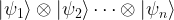
This is a good point in time to simplify our notation a bit. First, it is common to suppress the tensor product when it comes to states and to express the vector above simply as

$| \psi_1 \rangle | \psi_2 \rangle \dots | \psi_n \rangle$

Going further, we can also combine everything into one bra and write

$| \psi_1 \psi_2 \dots \psi_n \rangle$

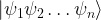
If we do this for the elements of a basis, we can simplify our notation even more. Let us do this for the states of a 2-qubit system first. By building tensor products of the base states $|0 \rangle$ and $|1 \rangle$ , we obtain four vectors

$|00 \rangle, |01 \rangle, |10 \rangle$ and $|11 \rangle$

These four states actually form a basis for the tensor product. This is true in general – all possible tensor products of the vectors of a basis are a basis of the tensor product space. Now recall that, in binary notation, the 2-bit sequences 00, 01, 10 and 11 stand for the number 0 – 3. Using this, we could also write this basis as

$|0 \rangle, |1 \rangle, |2 \rangle$ and $|3 \rangle$

For a three qubit system, we could use the same notation to arrive at the basis

and so forth. In general, for a combined system of n qubits, we can label our basis with the numbers 0 to 2ⁿ-1, and our tensor product will have dimension 2ⁿ, with a general element being given as a sum

$|\psi \rangle = \sum_0^{2^n-1} a_i |i\rangle$

Entangled states

To close this post, let us come back to one very important point that is a major ingredient to the theoretical power of quantum computing – entanglement. Suppose we are given a two-qubit system. We have seen that certain states can be obtained by taking the tensor product of single qubit states. Can every state in the tensor product be obtained in this way?

Let us try this out. If we take the tensor product of two arbitrary single qubit states $a |0\rangle + b |1 \rangle$ and $c |0\rangle + d |1 \rangle$ , we obtain

$ac |00\rangle + ad |01 \rangle + bc |10 \rangle + bd |11 \rangle$

Now let us consider the state

$| \psi \rangle = \frac{1}{\sqrt{2}} ( |00\rangle + |11 \rangle )$

To decompose this state as a product, we would need ad = 0 and ac = 1, which is only possible if d = 0. However, then bd = 0 as well, and we get the wrong coefficient for $|11 \rangle$ . Thus this is an example of a state which cannot be written as a tensor product of two single qubit states (but it can be written, of course, as a sum of such states). States that can be decomposed as a product are called separable states, and states that are not separable are called entangled states.

The state above is often called a Bell state and it is worth mentioning that states like this and entanglement features in one of the most famous though experiments in the history of quantum mechanics, the so called Einstein-Podolsky-Rosen paradox or ERP paradox – a broad topic that we will not even try to cover here. We note, however, that it is entanglement that is responsible for the fact that the dimension of the state space grows exponentially with the number of qubits, and most quantum algorithms use entangled states somehow, so entanglement does seem to play a vital role in explaining why quantum computing seems to be superior to classical computing, see for instance section 13.9 of “Quantum computing – a gentle introduction” for a more in-depth discussion of the role of entanglement in quantum algorithms.

Visualizing quantum states

Before closing this post and turning to quantum gates in the next post in this series, let us quickly describe a way how to visualize a multi-qubit quantum state. Our starting point is the expression

$|\psi \rangle = \sum_0^{2^n-1} a_i |i\rangle$

for the most general superposition in an n-qubit system. To visualize that state, we could use a bar char as in the diagram below.

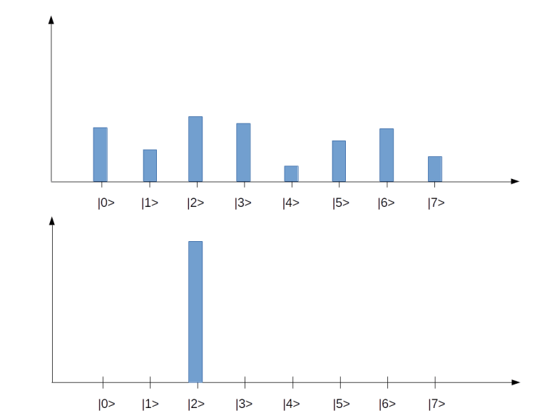
Each tick on the horizontal axis represents one of the basis states $|i \rangle$ . In our example, we have eight basis states, corresponding to a quantum system with 3 qubits. The bar represents the amplitude, i.e. the number $a_i$ in the superposition above (of course this is only a very incomplete representation, as it represents the amplitudes as real numbers, whereas in reality they are complex numbers). The upper state in the diagram represents a superposition for which all of the amplitudes are different from zero. The second diagram represents a state in which all but one amplitude is zero, i.e. a state that is equivalent to one of the basis vectors ( $|2\rangle$ in this case). These states correspond to the eight states of a corresponding classical system with three bits, whereas all states with more than one bar are true superpositions which have no direct equivalent in the classical case. We will later see how similar diagrams can be used to visualize the inner workings of simple quantum algorithms.

Qubits are nice, but in order to perform computations, we have to manipulate them somehow. This is done using quantum gates which I will discuss in my next post.

Networking basics – the TCP protocol

In our discussion of the IP protocol, the reader might have noticed that there are many desirable features that the IP protocol does not have. Suppose for instance that we are building an application that needs to transmit data in a stream oriented way – this could be a video, an MP3 file or a data transfer modelling a conversation. When we simply split our data into IP packets and send them directly via IP, there are many issues that we have to solve. IP does not guarantee us that packets even arrive, so we will have to deal with lost packets and build some acknowledgement and retransmission mechanism. Even if the packets arrive, the order in which they arrive is not guaranteed – different packets could be routed along different paths and arrive in reversed order. So we need a mechanism to encode the order and reassemble them at the destination in the right order. If the receiver needs some time to process the packets, we might want to control and dynamically adjust the rate of transmission. And finally, IP only assigns one address to a host (more precisely, a network card), so our transmission might conflict with other applications running on the same host and we need a way to deal with this.

Fortunately, the internet protocol stack offers a protocol sitting on top of IP and offering all this – the transmission control protocol, commonly known as TCP (there are other protocols on top of IP like ICMP that we have already seen in action and UDP, but we will focus on TCP in this post).

The main properties of the TCP protocol are:

It is reliable – the transmission of each piece of data is guaranteed by acknowledgement and retransmission capabilities of the protocol
It is connection oriented. When TCP is used, a connection with endpoints on both hosts is established first through a handshake procedure. Once the connection is established, both parties can write and read from the connection at the same time until all the data is transferred, then the connection is closed again. A connection endpoint (a socket) is identified using the IP address and an additional number, called the port number so that different connections originating or ending at the same host can operate independently.
It is stream oriented. An application dealing with TCP does not have to know anything about packet sizes, fragmentation, reassembly, MTUs and so forth – it just writes data sequentially into a socket or reads data sequentially from a socket. Most operating systems make writing to and reading from a socket as easy as dealing with a file. The protocol makes sure that the bytes that are written into one of the endpoints arrive at the second endpoint completely and in the same order.
And finally, TCP offers congestion control, i.e. the protocol automatically throttles the transmission speed if it realizes congestion.

TCP is a rather complicated protocol, and it is hopeless to cover it entirely in one post. Instead, we will look at a few of those points in more detail in the following sections.

Connection endpoints and ports

The TCP protocol has first been standardized in RFC 793 (and since then adapted and enhanced by many other RFCs). This is were we also find the structure of a TCP header (see section 3.1 of the document). The first two 16 bit words in the header are called source port and destination port.

Together with the IP address, the port number defines the full address relevant for a TCP connection. The combination of an IP address with a port number is sometimes called a socket in the RFC and is conventionally denoted by prefixing the port number by the IP address followed by a colon, for instance 192.168.178.1:23 for the port number 23 on the host with IP address 192.168.178.1. However, the port number does not simply supplement the IP address. Instead, TCP operates by building connections which are determined by the full endpoints – IP address and port numbers – on both sides.

Let us look at an example to explain this. Suppose you are running a web server on a host with IP address 10.0.2.20. Traditionally, a web server uses the port number 80.

Now suppose a first client connects to this web server. Let us assume that the client has the IP address 10.0.2.21 and that the operating system of the client decides to use the port number 3333 on the client to establish the connection (we will see below how exactly that works). When this connection is established, the web server will typically spawn off a separate thread to handle the communication with this client. So there is now one connection

10.0.2.21:3333 — 10.0.2.20:80

Now a second client might connect to the web server as well – of course we want this to be possible. If this client is running on a machine with IP address 10.0.2.22 and using port 3334, we obtain a second connection

10.0.2.22:3334 — 10.0.2.20:80

The situation is displayed in the image below.

The web server will create a second thread that serves HTTP requests that are placed using this connection. Now the point is that even though both connections share the same endpoint 10.0.2.20:80, they operate completely independently! If a TCP message arrives at port 80 of the web server, the operating system will inspect the source IP address and source port number to match the message to an existing open connection. It will then forward the message to the thread responsible for this connection and to no other thread. Thus a connection, identified by the quadruple IP source address, IP target address, TCP source port, TCP target port, serves as a channel through which data can flow independently of any other connections, even if they share a common endpoint. This makes TCP compatible with the paradigm of multi-threaded servers.

Handshakes and the TCP state machine

The connection based approach of TCP obviously requires a mechanism to establish a connection when the communication between two nodes begins. It also implies that a TCP connection has a state. This is a major difference between TCP and pure IP. In the IP protocol, every packet is treated the same – the processing of a packet is independent of any previously received packet (which is strictly speaking only true if we ignore fragmentation for a moment). For TCP, this is not true. A TCP connection has a state and the processing triggered by the arrival of a packet is in the context of that state.

Thus, from a theoretical point of view, a TCP connection can be described as a state machine. There is a (finite) number of states, and the connection will move from one state to the next state triggered by events and packets.

The full TCP state machine is rather complicated, and we will not discuss all possible transitions. Rather, we will focus on those transitions that a connection goes through until it is fully established. A graphical representation of this part of the state machine would look as follows.

To understand this image, let us go through the transitions and events one by one for a real world example. Suppose you are pointing your web browser to a specific site on the WWW, say http://www.wordpress.com. Your browser will then use a DNS service to turn this human readable address into an IP address, say 192.0.78.13. At this IP address, a web server is listening on port 80.

When this web server was started, it did ask the operating system on which it is running to reserve port 80 for it, so that it is automatically owning all incoming connections on this port. Technically, this is done using an operating system call called listen on most operating systems. The operating system now knows that the web server is claiming this port. It will establish an object called a socket and move this socket into the state “listening”. Thus, the endpoint on the server side does actually go through the transition at the top left of the image above – transitioning a connection from “closed” (i.e. not existing in this case) to “listening”.

You can use the command netstat -tln -4 on a Linux machine to get a list of all listening TCP connections (for IPv4). Depending on your configuration, you might see sockets listening on the ports 53 (DNS server), 445 (Microsoft Windows shares/CIFS), 80 (Web server) or 139 (Microsoft NetBios).

Back to our example – what is the web browser doing? After having resolved the IP address, it will try to establish a connection to the IP address / port number 192.0.78.13:80. To do this, it will assemble and send a special TCP packet called a SYN packet. This packet does not contain any data, but a special bit (the SYN bit) in the TCP header of this packet is set. After sending this packet, the client side endpoint is now in the state “SYN-SENT”, i.e. the client part of the connection did traverse the path on the upper right of our image.

Once the SYN packet arrives at the server side, the server will reply with a packet that has the acknowledgement bit set in its header, to let the client know that the SYN packet was received. It will then move into the next state – SYN-RCVD. As the SYN packet does contain the IP address and port number of the client, the server know knows the other endpoint of the connection.

Next, the client will receive the acknowledgement of the SYN packet. It will then reply with another acknowledgement, this time to let in turn the server know that is has received the servers acknowledgement. It then moves into the final state “ESTABLISHED”. Once the server receives the acknowledgement, it will do the same. At this point, the connection between both parties is fully established and the exchange of data can start.

Acknowledgement and retransmission

During the initial handshake, we have already seen an important mechanisms – acknowledgements. TCP is a reliable protocol, i.e. it guarantees that packets are received by the other endpoint. To make this work, each endpoint acknowledges receipt of all packets so that the sender knows that the data has been received. If a packet is not acknowledged within a certain period of time, it is retransmitted.

To allow for a retransmission, a sender needs to maintain a buffer of data which has been sent, but not yet acknowledged by the peer, so that the data is still available for retransmission. When data is eventually acknowledged, the part of the buffer containing that data can be emptied.

Conversely, the receiver will typically also have to maintain a buffer, as the application might need some time to read and process all the data. This raises another complication – how can we make sure that this buffer does not overflow? What we need is a mechanism for the receiver to inform the sender about the size of the available buffer. This is called the send window.

To explain these concepts in a bit more detail, let us take a look at the following diagram.

What we see here is a short piece of a longer stream of data that needs to be transmitted. Each of the little boxes is one byte of data, and the number within the box contains the offset of this byte within the stream. This number is reflected during the transition by a sequence number which is part of the header of a TCP packet and marks where in the stream the data within the packet is located. When a receiver acknowledges receipt of a packet, it adds the sequence number of the acknowledged data to the acknowledgement message to avoid a dependency on the physical order of packets.

To keep track of the stream status, the sender maintains two numbers. The first number, usually abbreviated as SND_UNA, contains the smallest sequence number that has been sent, but not yet acknowledged by the peer. Thus every byte with a smaller offset has been acknowledged and can safely be removed from the buffer.

The pointer SND_NXT contains the next sequence number that can be sent. Thus the bytes between SND_UNA and SND_NXT have been sent, but not yet acknowledged, and the bytes after SND_NXT have been passed to the operating system on the sender side, but not yet transmitted. If additional data is passed to the operating system for sending, they are stored in the buffer and SND_NXT is incremented. When an acknowledgement is received, SND_UNA is incremented and older bytes are removed from the buffer.

An additional restriction is now given by the size of the send window. During the initial handshake, both endpoints exchange their desired send windows. The send window is then used as an upper bound for the number of bytes that are allowed to be in transit. Thus, in the example above, the bytes starting at offset 110 have already been handed over to the operating system for sending, but are in fact not yet ready to be sent as the send window of the peer is only 10 bytes.

All this sounds still comparatively simple, but can in fact become quite complicated. Complex algorithms have been defined in several RFCs to determine when exactly data is to be sent, what happens if an acknowledgement is not received, when exactly acknowledgements are sent, how the send rate is to be adapted to the capacity of the connection (congestion control) and so forth. Discussing all this would go far beyond the scope of this blog post. For those interested in the details, I recommend the two volumes of TCP/IP Illustrated by W. R. Stevens. If you prefer to look at source code, there are the implementations in the open source operating systems like FreeBSD and Linux. In addition, there is the implementation that I coded for my own toy operating system, especially the documentation of the networking stack and the source code of the TCP module.

Quantum computing

When I started this blog, my intention was to document my own attempts to learn and understand some of the topics at the intersection of computer science, physics and mathematics that have the potential to change the world in which we work and live. After spending some time with one of these topics – machine learning and artificial intelligence – I have now started to look into one of the most exciting combinations of these subjects – quantum computing.

Roughly speaking, quantum computing refers to leveraging the laws of quantum mechanics – like superposition and entanglement – to build computing devices that operate in a way fundamentally different from traditional computers and allow us to solve traditionally hard computational problems in a reasonable amount of time.

How exactly this works is difficult to explain without referring to non-trivial quantum mechanics and mathematics. It is often said that quantum computing is exploiting the superposition principle – the fact that the state of a quantum system can be described as a superposition of many different fundamental states at the same time – to perform many calculations parallel in one step that a classical computer can only perform serially. However, we will see that this is a bit of an oversimplification as it ignores the fact that a measurement destroys this parallelism.

In addition, even though a quantum computer is theoretically able to perform any calculation that a classical computer can do, it is not clear that we will see a drastic speedup for arbitrarily chosen classically hard problems. In fact, as of today, we know a few problems – like the factorization of large composite numbers into primes – that can be solved using quantum computers while being intractable for traditional hardware, and we know of some areas of applications like simulations or optimization and machine learning, where we have good reasons to expect that quantum computing will provide a massive gain in speed and capacity, but there is strong evidence that not all classically hard problems can be solved efficiently on a quantum computer (see for instance [1]). And sometimes, we find a fast quantum algorithm for something that so far could not be done efficiently on a classical computer, but this algorithm then inspires a classical solution providing the same speedup (the recommendation problem seems to be an example for that fruitful interaction between quantum computing and classical computer science).

So even a fully operational universal quantum computer would not out of a sudden make classical computing obsolete and perform better in all known instances. Rather, we should expect that at least in the near future, the main applications of quantum computing will be restricted to a few dedicated fields, with classical computing evolving in parallel (see for instance [2] for a discussion).

This does not make quantum computing less exciting. After all, quantum computing changes the way how we think about things like information and algorithms substantially. However, implementing a working quantum computer remains hard. In later posts, we will look at some of the technologies like quantzum error correction, superconducting devices and ion traps that are currently used by researchers around the globe to build quantum computing devices at scale. We have seen some very exciting progress recently, with e.g. Google announcing its new Bristlecone device with 72 qubits or IBM making a 5 qubit quantum computer publicly accessible in the cloud as part of their Q Experience program. There are even simulators like Quirk that allow you to put together quantum circuits online and play with the results or frameworks like Microsofts quantum development kit or the API and framework developed by 1QBit that support the development and debugging of quantum algorithms before trying them on a real quantum device. So it is definitely a good point in time to get to know some of the basics of quantum computing, covering theory, applications and implementation – and this is the goal of this new series.

Currently, my plans are to cover the following topics in the upcoming posts.

- Fundamentals: qubits and Hilbert spaces
- Quantum gates and unitary transformations
- Grover’s search algorithm
- Quantum Fourier transform
- Shors algorithm
- The quantum variational eigensolver
- Simulation
- Error correction – basics, fault tolerant quantum computing, stabilizer codes, toric codes and surface codes
- Superconducting quantum devices
- NMR based quantum computers
- Playing with IBMs Q experience – first steps, the Python API, the Deutsch-Jozsa algorithm and the Quantum Fourier Transform
- Factoring integers using Shor’s algorithm and IBMs Q experience
So in the next post, I will set out explaining what a qubit is and how a qubit is described in the language of quantum mechanics and mathematics. Until then, I recommend the links below which provide some selected reading on applications and limitations of quantum computing as of today.

1. C.H. Bennet, E. Bernstein, G. Brassard, U. Vazirani, Strengths and Weaknesses of Quantum Computing, arXiv:quant-ph/9701001v1
2. J. Preskill, Quantum Computing in the NISQ era and beyond, arXiv:1801.00862
3. Finding Optimal Arbitrage Opportunities Using a Quantum Annealer, http://www.quantumforquants.org/quantum-computing/qa-arbitrage/
4. The excellent Wikipedia article on quantum machine learning
5. Job One for Quantum Computers: Boost Artificial Intelligence
6. The Era of Quantum Computing Is Here. Outlook: Cloudy

Networking basics – IP routing and the ARP protocol

In the last post in this series, we have covered the basics of the IP protocol – the layout of a network message and the process of fragmentation. However, there is one point which we have not yet discussed. Assume that an application or operating system has actually assembled a message and applied fragmentation so that the message is now ready to be sent. How would that actually work?

Routing in local networks: the ARP protocol

To understand the situation, assume for a moment that we are dealing with a very simple network topology. We are looking at a host which is part of a small network, and the host is directly connected to the same Ethernet network segment as the destination host, as illustrated in the following diagram.

Here we are considering a network consisting of a small number of workstations and one Ethernet switch (in the middle of the diagram). Each workstation is equipped with a network interface card (NIC) which has an Ethernet (MAC) address. Thanks to the switch, Ethernet frames sent out by one NIC can be directly read by any other NIC.

At configuration time, each NIC receives an assigned IP address. This is usually done using a technology like DHCP, but can also be done manually as long as no IP address is used twice.

Now suppose that the workstation with IP address 192.168.178.2 (more precisely: the workstation to which the network interface card with assigned IP address 192.168.178.2 is attached) wishes to send an IP packet to the workstation with IP address 192.168.178.3. It then needs to make several decisions:

which network interface card should be used to transmit the packet?
which Ethernet target address should be used?

In the simple case that we consider, the answer to the first question is obvious, as there is only one NIC attached to the workstation, but this question will become more relevant in the more complex setup that we will study later. The second question is more interesting – to answer it, the workstation somehow needs a way to translate an IP address into the MAC address of the corresponding NIC.

To do this, the ARP protocol is at our disposal. ARP is the abbreviation for Address resolution protocol and is defined in RFC 826. ARP messages are designed to travel on top of Ethernet or other link layer protocols. Essentially, the ARP protocol is request-reply based. If a host wishes to translate an IP address into an Ethernet address, it will send an ARP request to all hosts on the local network, using an Ethernet broadcast. This message will contain the own IP and MAC address and the IP address that the host is looking for. Each host on the network will compare the IP address to its own IP address. If they match, it will respond with a reply message that again contains the own IP and MAC address. The requesting host can then use this message to retrieve the correct MAC address and use it for further communication.

Of course this procedure is not repeated every time a host wants to send a packet to another host in the local network. Instead, a host will cache a mapping of IP addresses to Ethernet MAC address in a so called ARP cache. As the assignment of IP addresses to network interface cards can vary over time, entries in this cache typically have a timeout so that they become invalid after some time. On a Linux workstation, the arp command can be used to print the current content of the ARP cache, i.e. the set of hosts to which the workstation has a direct connection that has been recently used. On my PC, the output looks as follows.

$ arp -n
Address                  HWtype  HWaddress           Flags Mask            Iface
192.168.178.1            ether   08:96:d7:75:7e:80   C                     enp4s0
192.168.178.33           ether   ac:b5:7d:34:3a:a6   C                     enp4s0
192.168.178.28           ether   00:11:32:77:fe:46   C                     enp4s0

Here we see that the network card of my PC is able to connect directly to three other hosts on the same Ethernet network. The first one is my router, the second one is a laptop connected to the same router via WLAN (the router actually contains a switch that makes the devices connected via WLAN to appear on the network as an Ethernet device) and the third one is a NAS.

Summarizing, here are the steps that a host would typically take to send an IP packet to another host on the local network.

Look up the target IP address in the ARP cache
If there is a match, retrieve the MAC address from the ARP cache entry, assemble an Ethernet frame with that target address and send it
If there is no match, send an ARP request as broadcast into the local network. Once a reply arrives, add a corresponding entry to the ARP cache. Then proceed as above by assembling and sending the Ethernet frame
If no ARP reply arrives, give up – this will typically result in an error message like “destination host unreachable”

Note that the ARP protocol is designed to determine the target Ethernet address inside a local network. ARP requests will be dropped at network boundaries. Now, the Internet is by design a network of network – it consists of many small networks that are connected to each other. Obviously, the ARP protocol is no longer sufficient to solve the routing challenge in these more complex networks, and we need additional tools. This will be discussed in the next section.

Routing across network boundaries

For the sake of concreteness, let us again take a look at a slighly modified version of the example network that we have already used earlier in this series.

In this example, our entire network is comprised of three different networks, called network 1, network 2 and network 3. In each of these networks, each host is reachable from any other host directly via an Ethernet medium. Thus for the communication within each of these networks, the mechanisms explained in the previous section apply – a host uses the ARP protocol to translate IP addresses into MAC addresses and sends IP messages directly as payload of Ethernet frames.

Now let us walk through the chain of events that takes place when in this topology, host B wishes to send an IP packet to host A. The first thing that host B needs to detect is that host A is not part of the same Ethernet network. To be able to do this, an additional configuration item is used that we have ignored so far – the subnet mask.

When a network interface card is set up, we typically do not only assign an IP address to it, but also a network mask. Technically speaking, a network mask is – as the IP address itself – a sequence of four bytes, using the same decimal dot notation that we use for the IP address. Thus, as the IP address, it is a sequence of 32 bits. We can therefore apply a boolean AND operation to the IP address and the network mask. The result is, by definition, the network part of the IP address, the remaining part is the host part of the IP address. All IP addresses which share a common network part are considered to be part of the same subset, and the standard IP routing algorithms assume that they are connected directly via Ethernet or another link layer protocol.

Let us look at an example to make this clearer. In our case, the network mask for all three subnets is 255.255.255.0. When we take the IP address 192.168.1.3 of host B and apply a logical AND to this and the network mask, we obtain the network part 192.168.1.0, as displayed in the table below.

When we apply the same procedure to host A, we obtain the network 192.168.3.0. Thus the two hosts are not in the same subnet, and host B can use that information to determine that a direct routing attempt via ARP will not work (this is actually a bit of a simplification – typically, the host will use an algorithm known as longest match prefix algorithm involving the network mask).

Instead, in order to reach host A, host B will have to make use of a so-called gateway or router. Roughly speaking, a gateway is a host that is connected to more than one network and can therefore transmit or route (hence the name router which is often used as a synonym, even though this is not entirely correct, see RFC 4949 for a discussion of the terminology) packets between the networks.

In our example, there are two gateways. The first gateway connects the networks 1 and 2. It has two network interface cards. The first NIC is connected to network 1 and has the assigned IP address 192.168.1.1. The second NIC attached to this host is part of network 2 and has the assigned IP address 192.168.2.2 (this example makes it clear that, strictly speaking, the IP address is not an attribute of a host but of the network interfaces attached to it).

When host A wishes to send an IP packet to host B, it will send the packet to this gateway via the NIC attached to network 1. As this NIC is on the same Ethernet network, this can be done using the ARP resolution protocol discussed earlier. The gateway will then inspect the destination IP address of the packet and consult a table of possible next stations called the routing table. Based on that table, it will decide that the best next station is the gateway connecting network 2 and network 3. This gateway will finally determine that the destination IP address is part of network 3 to which it is directly attached and eventually deliver the packet to host B.

Thus our IP packet did have to pass several intermediate hosts on its way from source to destination. Each such host is called a hop. The traceroute utility can be used to print out the hops that are required to find a way to a given destination address. Essentially, the way this utility works is as follows. It will send out sequences of packets (typically UDP) towards a given destination, with increasing value of the TTL (time-to-live) field. If the value of this field is n, it will only survice n hops, until it will be dropped. The host dropping the packet will send an ICMP packet back to the host on which traceroute runs. This ICMP packet is used by the utility to determine that the sender of the ICMP packet is part of the route and is sitting at station n in the route. By increasing the TTL further until no packets are dropped anymore, the entire route to the destination can be probed in this way.

Here is the output of a traceroute on the workstation on which I am writing this post.

$ traceroute www.wordpress.com
traceroute to www.wordpress.com (192.0.78.13), 30 hops max, 60 byte packets
 1  fritz.box (192.168.178.1)  2.289 ms  3.190 ms  5.086 ms
 2  dslb-178-004-200-001.178.004.pools.vodafone-ip.de (178.4.200.1)  22.503 ms  24.686 ms  25.227 ms
 3  * * *
 4  * * *
 5  92.79.212.61 (92.79.212.61)  33.985 ms 92.79.212.45 (92.79.212.45)  35.649 ms  36.373 ms
 6  145.254.2.175 (145.254.2.175)  38.205 ms 145.254.2.191 (145.254.2.191)  23.090 ms  25.321 ms
 7  edge-a01.fra.automattic.net (80.81.193.69)  25.815 ms  18.981 ms  19.729 ms
 8  192.0.78.13 (192.0.78.13)  22.331 ms  19.813 ms  19.593 ms

We can see that the first station in the path to the destination http://www.wordpress.com is my local DSL router (192.168.178.1), which, not surprising, acts as a default gateway for my local home network. The DSL router than forwards the packet to the next hop (178.4.200.1), which, judging by its name, is part of the DSL infrastructure of my ISP (Vodafone). The next two lines indicate that for the packets with TTL 3 and 4, the utility did not get an answer, most likely because some firewalls were preventing either the probing UDP packet from reaching its destination or because the ICMP message was not sent or not received. Finally, there are three more hops, corresponding to the TTL values 5,6 and 7, before the final destination is reached.

This sounds simple, but in fact routing is a fairly complex process. In a home network, routing is comparatively easy and the routing table is fairly short (you can use the command route on a Linux system to print out the routing table of your machine). Typically, there are only two entries in the routing table of an ordinary PC at home. One entry tells the operating system that all packets that are targeted to an IP address in the local network are to be sent to the local network interface without any gateway. The second entry is the so-called default gateway and simply defines that all other entries are to be sent to a default router, which is for instance the cable modem or DSL router that you use to connect to your ISP.

However, once we leave a home network, life becomes more complicated as there is typically more than one possible path from a source host to a destination host. Thus a host might have more than one possible choice for the next hop, and a lot hinges on routers correctly building their routing tables. Several routing protocols exist that routers use to exchange information among each other to find the best path to the destination efficiently, like ICMP, OSPF, BGP or IS-IS, see RFC 1812, RFC 1142 or RFC 1247 for more details.

There are many topics related to IP networking and routing that we have not yet discussed, for instance network address translation (NAT), details on the ICPM protocol, CIDR notation and address classes, and IP version 6. Instead of getting further into these details, however, we will devote the next post in this series to a protocol sitting on top of IP – the TCP protocol.