Bulk quantum computing with nuclear spin systems

The theoretical foundations of universal quantum computing were essentially developed in the nineties of the last century, when the first native quantum algorithms and quantum error correction were discovered. Since then, physicists and computer scientists have been working on physical implementations of quantum computing. One of the first options that moved into the focus was to use a technology known as nuclear magnetic resonance (NMR) to develop universal quantum computers. In this post, we give a brief overview of NMR based quantum computing and prepare to dive into some advanced topics in the next few posts.

Introduction to NMR

Nuclear magnetic resonance is not a new technology. It was already developed to a high degree when quantum computation was initially discussed, and was therefore a natural choice for first implementations.

So what is NMR? Recall that all matter (as we know it) consists of molecules which, in turn, are compounds of atoms. Each atom consists of a nucleus and a cloud of electrons.

A nucleus is itself not an elementary particle, but is a composite system, formed by protons and neutrons (which again are not elementary but consist of quarks). As every elementary particle, each constituent of a nucleus has a spin degree of freedom. These spins add up to a total spin. Of course, the spin depends on the quantum mechanical state of the nucleus, but typically, the energy gap between the ground state and the first excited state is so high that at room temperature, it is a good approximation to assume that the spin of the nucleus is the ground state spin. The value of this spin of course depends on the structure of the nucleus. Some nuclei, like deuterium, have spin one, some – like ¹²C have spin zero, some like ¹³C have spin 1/2, and some have higher spins.

Of course the nuclear spin interacts with an external magnetic field. The strength of this interaction is determined by the coupling between the magnetic field and the spin which is expressed by the gyromagnetic moment of the nucleus.

Now suppose we are given a probe of a substance with nuclear spin 1/2 that is subject to an external field along some axis, say the z-axis. Let us simplify the discussion a bit by looking at a single nucleus only and ignoring all spatial degrees of freedom. The nuclear spin is then described by a two-level system, i.e. a qubit. The Hamiltonian of this system is

where is the gyromagnetic moment, B is the magnetic field in the z-direction and is the usual Pauli Z-operator, i.e. the Hamiltonian is simply a multiple of the Pauli Z operator. Consequently, the time evolution operator is

with . Thus, on the Bloch sphere, the time evolution is a rotation around the z-axis with frequency . This rotation is called the Larmor precession and the frequency is called the Larmor frequency. For typical nuclei and fields, the Larmor frequency is in the order of a few hundred MHz.

Let us now suppose that the spin is originally in the ground state, i.e. pointing to the north pole of the Bloch sphere.

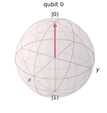
What happens if we now apply an external additional magnetic pulse? The answer will obviously depend on the frequency and direction of the pulse. A detailed analysis that we will carry out in a later post shows that if the frequency of the pulse is equal to the Larmor frequency, the effective Hamiltonian during the pulse (in a rotating frame of reference) is proportional to the Pauli X matrix. Therefore the time evolution operator during the pulse corresponds to a rotation around the X-axis. If we time the pulse correctly so that the angle of this rotation is , then the nuclear spin will flip into a direction perpendicular to the z-axis.

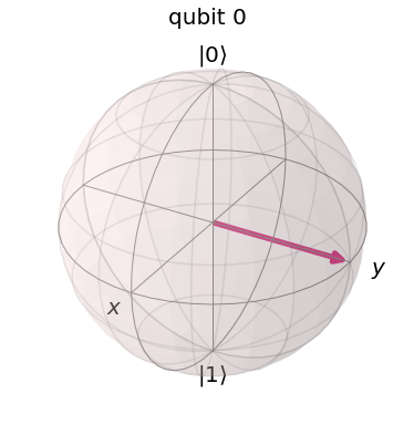
After the pulse has completed, the time evolution is now again given by the rotation around the z-axis with the Larmor frequency. Consequently, the spin axis will start to precess around the z-axis. This spin precession represents a rotating magnetic moment and creates an oscillating magnetic field which in turn can be detected by placing a coil close the probe so that the rotating field will induce a voltage in the coil. Of course, the frequency of the observed signal will be that of the rotation, i.e. the Larmor frequency of the nucleus in question. We therefore find that we obtain a resonance peak at the Larmor frequency if we slowly vary the frequency of the external pulse.

In a probe that contains several different types of nuclei, we will observe more than one resonance peak – one at the Larmor frequency of each of the involved nuclei. The location and relative strength of these peaks can be used to determine the nuclei that make up the probe, and can even yield insights into the interactions between the nuclei and therefore the structure of the molecule. This technique is called nuclear magnetic resonance (NMR).

How NMR can be used for quantum computation

This description of the NMR process is on a very heuristic level, but it can be made precise (and we will look at a few more details in the next few posts). But let us take this for granted for today and let us discuss how this technology can be applied to implement a universal quantum computer.

At the first glance, this looks like a perfect match. If we pick a nucleus like ¹³C which has spin 1/2, the spin degree of freedom is described by a two-level system which makes for a perfect qubit. We have already indicated above that rotations on the Bloch sphere, i.e. one-qubit operations, can be realized by applying correctly timed magnetic fields. Given that the NMR technology is already highly developed, it appears that NMR should be a good candidate for an implementation.

However, there are few subtleties that we have ignored. First, we have not yet discussed multi-qubit systems. Of course, in a typical molecule, there is more than one nucleus. Not all nuclei have spin 1/2, but for some molecules, we will find several spin 1/2 nuclei which could serve as qubits. In one of the first applications of NMR to quantum computing (see [3]) for instance, a custom designed molecule was chosen to represent five qubits. Of course, this method is difficult to scale if we want to build systems with more than 20 or 50 qubits, but for a low number of qubits, it has been demonstrated to work.

Another problem which we have largely ignored so far is that of course, the probe that we use consists of a very large number of molecules. When we place this probe in our external magnetic field, the spin axis of the individual nuclei will not point all in the same direction, but instead we expect a random pattern of spin orientations. How can we then prepare the system in a well defined initial state? And how can we avoid that the individual signals created by each qubit cancel each other completely because of the random orientation of the spin axis? Of course we could try to cool down the system to a very low temperature to force all spin nuclei into the ground state, but this would make dealing with the system difficult and take very long. A solution to this problem was presented in [4] and [5] – it turns out that even though it appears almost impossible to prepare the system in a pure state, one can prepare it in a state which has properties similar to a pure state and is sufficient to do quantum computation.

In fact, the NMR technology quickly turned into the technology of choice for the first experimental verifications of quantum algorithms due to the availability of high-resolution NMR spectrometers and the many years of experience in the field. The first-ever factorization of an integer on a quantum computer using Shor’s algorithm (albeit a toy version which only works because the result was known upfront, see also my previous post on realizing Shor’s algorithm with Qiskit) was done on an NMR computer (see [6]). In recent years, however, other technologies like superconducting qubits and ion traps have moved more into the focus of the various research groups. Nevertheless, NMR based quantum computing is worth being studied as it illustrates many of the basic principles of the field.

This completes our short overview of NMR based quantum computation. In the next few posts, we will dig deeper into some of the questions raised above, starting with a more precise description of the physics underlying a single qubit NMR based quantum computation.

References

1. M.H. Levitt, Spin dynamics – basics of nuclear magnetic resonance, John Wiley & Sons, 2008
2. D.P. DiVincenzo, The Physical Implementation of Quantum Computation, arXiv:quant-ph/0002077
3. L.M.K. Vandersypen et. al., Experimental realization of order-finding with a quantum computer, arXiv:quant-ph/0002077
4. D.G. Cory, A.F. Fahmy, T.F. Havel, Ensemble Quantum Computing by NMR Spectroscopy, Proceedings of the National Academy of Sciences of the
United States of America, Vol. 94, No. 5 (Mar. 4, 1997), pp. 1634–1639
5. N.A. Gershenfeld, I.L Chuang, Bulk Spin-Resonance Quantum Computation, Science Vol. 275, Jan. 1997
6. L.M.K. Vandersypen et. al., Experimental realization of Shor’s quantum factoring algorithm using nuclear magnetic resonance, Nature Vol. 414, Dec. 2001