March 2019 – LeftAsExercise

Quantum error correction: an introduction to toric codes

While playing with the IBM Q experience in some of my recent posts, we have seen that real qubits are subject to geometric restrictions – two-qubit gates cannot involve arbitrary qubits, but only qubits that are in some sense neighbors. This suggests that efficient error correction codes need to tie to the geometry of the quantum device. Toric codes are an example of these codes that create interesting connections between topology and quantum computing.

The stabilizer group of a toric code

In their original form introduced by A. Kitaev in 1997 (see e.g. [1]), toric codes are designed to operate on quantum circuits arranged on a torus. Specifically, we consider a 2-dimensional discrete lattice L with periodic boundary conditions. On each edge of this lattice, we place exactly one qubit.

In algebraic topology, one can associate with such a lattice an abelian group called the group of one-chains of the lattice and denoted by $C_1(L)$ . The elements of this group are simply binary linear combinations of edges, i.e. subsets of all edges. Addition in this group is given by joining the subsets, while dropping elements that appear twice. As there is one qubit sitting on every edge, every chain c, i.e. every subset of edges, will yield an operator that we call X_c and which is simply given by applying the Pauli X operator to each of the qubits sitting on an edge appearing in c. Similarly, one can define an operator Z_c for evey chain c by combining the Pauli Z operators for the qubits touched by c.

This sounds a bit daunting and formal, so time to look at a picture and a few examples.

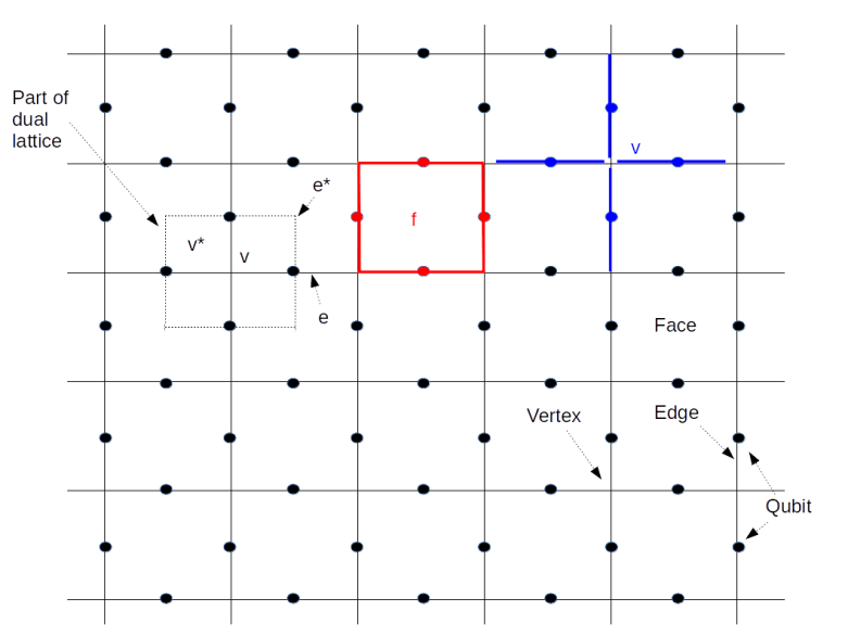
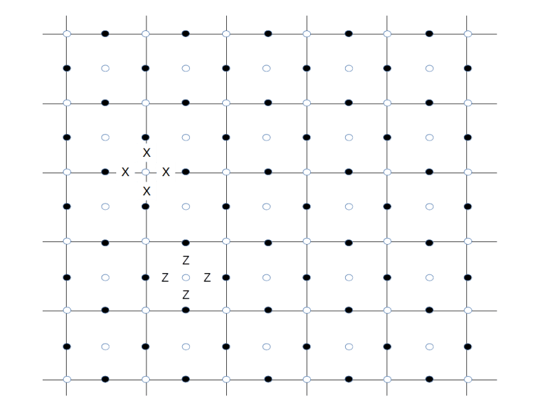
This diagram shows a graphical representation of our lattice L. The solid lines represent the edges of the lattice, their intersections are the vertices, see the labels at the lower right corner of the image. Cornered by four vertices and surrounded by four edges, there are the faces of the lattice. The black dots in the diagram indicate the qubits on the lattice.

Now let us look at the face marked in red and labeled by f at the top of the diagram. This face is surrounded by four edges colored red as well whose union is called the boundary of the face. This boundary is formalized as a one-chain denoted by $\partial f \in C_1(L)$ . As described above, we can associate an operator $Z_{\partial f}$ to this one chain, which is simply given by letting a Pauli Z operator act on each of the qubits sitting on the red edges. This operator is called the face operator associated with the face f and denoted by Z_f

On the right of the face, we have – in blue – marked a single vertex v. This vertex again defines a chain, namely the subset of all edges – marked in blue – that touch the vertex. Again, we can associate an operator to this chain, this time we choose the product of the Pauli X operators acting on the qubits on the blue edges. This operator is called the vertex operator for the vertex v and denoted by X_v.

Our lattice has many faces and many vertices. For each face, we have a face operator and for each vertex, we have a vertex operator. It is not difficult to check that all these operators do in fact commute (note that a vertex touches every boundary twice). Therefore the group S generated by all these operators is an abelian group.

Now recall from one of my previous posts that the stabilizer formalism can be used to associate to every abelian subgroup of the Pauli group a code. The code obtained from the group S generated by all face and vertex operators is called the toric code.

Let us try to better understand the code space T_S. Suppose that our lattice has E edges, V vertices and F faces. Then there are E qubits, i.e. the Hilbert space of physical qubits has dimension 2^E. The stabilizer group is generated by the V vertex operators and the F face operators, i.e. by V + F elements. However, these elements are not independent – there are relations imposed by the toric geometry. In fact, the product of all vertex operators is one and the product of all face operators is one (this is easiest seen with a bit of background in algebraic topology – for those readers who have that background, I refer to my notes on quantum error correction for the mathematical details behind this and some other statements in this post). Thus there are in fact V + F – 2 generators. As each generator introduces a constraint on the code space that cuts the Hilbert space dimension down by a factor two, the dimension of the code space is

2^{E – (V+F – 2)} = 2^{2 – (V + F – E)}

Now the number V + F – E is known as the Euler number of the torus in algebraic topology, and it also known that the Euler number of the torus is zero. Therefore the dimension of the code space is 2² = 4, i.e. the code space encodes two logical qubits (this will change if we later move on to a planar geometry).

Let us now try to understand the logical gates acting on these two logical qubits. By the general theory of stabilizer codes, we know that the logical operators are those operators that commute will all elements in the stabilizer. What does this mean geometrically? To see this, consider the following diagram.

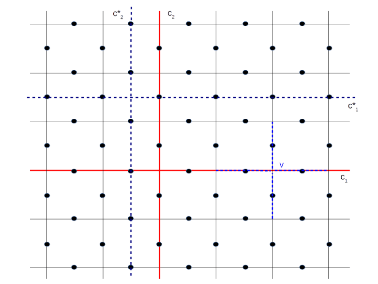
Consider the vertical red line in the diagram, labeled by c₁. This line is a subset of edges, i.e. a one chain. To this chain, we can associate a Z operator Z_c₁, which is the product of all Pauli Z operators acting on the qubits touched by the red line. Being a Z operator, this operator commutes with all face operators. What about the vertex operators?

Close to the right border of the lattice, we have indicated the vertex operator X_v associated with the vertex v. This vertex operator acts on four qubits, indicated by the edges marked with the blue dashed line. Two of these edges also appear in the chain c₁. Therefore, when we commute X_v and Z_c₁, we pick up two signs that cancel and the operators commute. Thus Z_c₁ commutes with all vertex and face operators and is in the normalizer. The same is true for the operator associated with the second red line. These two Z operators therefore act on the logical qubit. By convention, we can define the logical state $|0 \rangle_L$ to be the state which is left invariant by these two operators.

It is interesting to note that the vertex operator X_v commutes with Z_c₁ because the chain c₁ crosses the vertex v and therefore contains both edges touching v. If however, a chain c ends at v, then we will only pick up one sign when commuting the X past the Z operators. Geometrically, a vertex operator X_v anti-commutes with a Z-operator Z_c associated with a chain c if and only if the vertex v is in the boundary of c, otherwise it commutes. The red line in our diagram is distinguished by the fact that its boundary is empty – it is a closed circle or a cycle in the language of algebraic topology that goes around the torus once. It therefore commutes with all vertex operators and thus is an element of the stabilizer.

Similarly, the dotted blue lines represent X operators, given by the product of the Pauli X operators acting on those qubits intersected by the blue line. A similar argument shows that, as these lines also go once around the torus, the X operators associated with them are in the normalizer of S as well. Thus we obtain two X operators that act as logical Pauli X operators on our code space. Given the logical X and Z operators, we can therefore implement all single qubit gates on our code space. It turns out that multi-qubit gates can be implemented by braid operations, but we will leave this to a later post when we study planar codes.

The particle interpretation of the toric code and anyons

Let us now turn to the particle interpretation of error correction in these codes, that will bring the famous anyons and ideas from topological quantum computing into play. For that purpose, consider the operator

$H = - \sum_v X_v - \sum_f Z_f$

which is the sum of all face and vertex operators. Clearly, this operator is hermitian, and can therefore be thought of as the operator of a physical system. Does this system have a particle interpretation?

To see this, let us try to determine the eigenstates of the Hamiltonian, i.e. the energy levels of our system. As the X_v and the Z_f all commute, we can find a simultaneous basis of eigenstates that will diagonalize the Hamiltonian. Let us call this basis $\{ |\psi_i \rangle \}$ . Each of these vectors is an eigenstate of all face and vertex operators, and we denote the corresponding eigenvalues by x_vi and z_fi. Clearly, $|\psi_i \rangle$ is then an eigenvector of H with eigenvalue

$- \sum_f z_{fi} - \sum_v x_{vi}$

This is minimal if and only if all the x_vi and z_fi are equal to one, which is the case if $|\psi_i \rangle$ is an element of the code space. Thus we have identified the elements of the code space as the ground states of our system!

Now let us introduce an error into our system. One way to do this is to pick a chain c, i.e. a path on the lattice, and apply the Z_c operator to one of the ground states $|g \rangle$ . Let us try to determine the error syndrome of this state, i.e. let us try to figure out for which elements of the stabilizer, this state is no longer in the +1 eigenspace.

As all Z operators commute, the state is clearly still in the +1 eigenspace of all the face operators Z_f. If X_v is a vertex operator, the state will be in the -1 eigenspace if and only if Z_c anti-commutes with X_v. But we have already seen that this happens if and only if v is in the boundary of c, i.e. v is one of the two vertices where the path c starts and ends! Thus the error syndrome is localized at those two vertices – if we imagine the vertex operator measurements as being signaled by green (outcome plus one) and red (outcome minus one) lights attached to the respective vertex, the error would be represented two red lights sitting at these vertices.

If we now expand the state $Z|g \rangle$ into eigenstates of the Hamiltonian, the above discussion shows that the eigenvalue has increased by four. Thus errors correspond to excited states, and the operators Z_c are creation operators that create excited states that are in a certain sense localized at the vertices of the lattice. It is tempting and common to therefore call these excitations quasi-particles, similar to the phonons in a crystal lattice.

So far we have associated an error operator Z_c and therefore a particle with every chain, i.e. a path that runs along the edges. We can also consider a path that runs perpendicular to all the edges – in algebraic topology, this would be called a chain in the dual lattice or a co-chain. To every such path, we can associate an X operator, and this X operator acting on a ground state will create another excitation. The particles associated with a chain is called an electric charge e by Kitaev, and the particle created by a co-chain is called an magnetic vortex m.

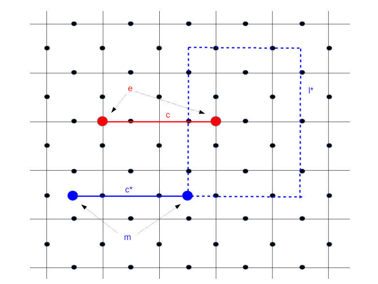
As indicated in the diagram above, electric charges come in pairs, are located on vertices of the lattice and manifest themselves as -1 eigenvalues of the corresponding vertex operators, whereas magnetic particles live on pairs of faces of the vertex and appear as -1 eigenvalues of face operators. In this diagram, the solid red line creates a pair of electric particles, and the solid blue line creates a pair of magnetic particles.

How do these particles relate to the composition of chains? Suppose that we are given a chain c₁₂ running from vertex 1 to vertex 2 and a second chain c₂₃ running from vertex 2 to vertex 3. Then there are two ways to create the particle sitting at the vertices 1 and 3 – we can either first act with the Z operator associated with the chain c₁₂ and then let the operator associated with the chain c₂₃ act, or we can form the sum c₁₃ of the chains which now runs from 1 to 3 and let the operator associated with this chain act. Of course, the result will be the same. Thus we can interpret the act of applying the operator given by the chain c₂₃ to an excited state as moving one of the particles from vertex 2 to vertex 3. The same applies to magnetic particles.

Now let us again consider the image above. Look at the blue dashed loop. According to what we have just said, we can start with the particle pair created by the solid blue line and then move one of the particles around that closed loop. The result will be a particle pair living at the same location as the original pair. You might think that the new state is in fact identical to the old state, but this is not true – the state picks up a phase factor minus one. This is the reason why Kitaev calls our quasi-particles anyons, a term generally used in particle physics to characterize particles with non-trivial statistics (in our case, mutual statistics)

Exchanging particles by moving them around each other can be described as an action of the pure braid group, i.e. as an action of the group of braids that return each particle to its original position (this subgroup, the kernel of the natural homomorphism from the braid group to the permutation group, is sometimes called the group of colored braids). If we perturb a braid slightly, the action will remain unchanged, so the unitary operators which are given by that action are by construction rather stable in the presence of noise. In [1], Kitaev developed the idea to use braid group representations to implement quantum gates. Unfortunately, the set of operators that we can obtain in this way using the toric code is not sufficient to implement a universal quantum computer – we will get back to this point in a later post when we look at the actual procedures used to perform computations in a toric or surface code. Therefore Kitaev goes on to describe certain hypothetical particles called non-abelian anyons which, if they can be physically realized, provide sufficiently rich unitary operations. This approach is called topological quantum computation. We will not go into further details but refer to the original work [1].

Measurement and error correction for toric codes

Let us quickly summarize what we have found so far. The code space of a toric code can be thought of as the ground state of a physical system, describing a collection of two-state systems located on the edges of a lattice. Errors correspond to fundamental excitations, i.e. quasi-particles, that come in pairs and sit on vertices and faces of the lattice. These errors can be detected by measuring face and vertex operators.

How can we perform these measurements in practice? To understand this, let us first recall a general approach for measuring eigenvalues. Suppose that U is an operator that is hermitian and at the same time unitary. Consider the following circuit which is a combination of two Hadamard gates with a controlled-U operation.

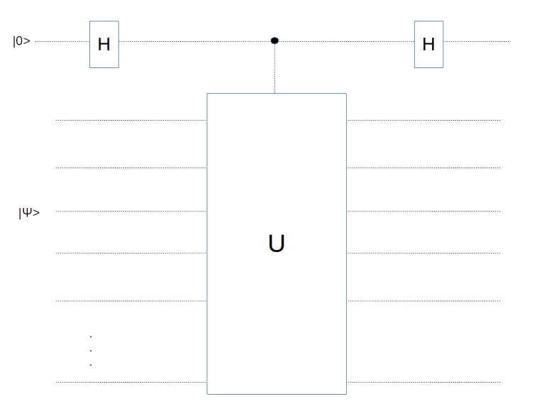
Let us calculate the state after applying this circuit. The initial state is

$|0 \rangle |\psi \rangle$

After applying the Hadamard gate to the first qubit, we obtain

$\frac{1}{\sqrt{2}} \big[ |0 \rangle |\psi \rangle + |1 \rangle |\psi \rangle \big]$

which the controlled U operation turns into

$\frac{1}{\sqrt{2}} \big[ |0 \rangle \otimes |\psi \rangle + |1 \rangle \otimes U |\psi \rangle \big]$

Now U is unitary, and therefore its eigenvalues are plus and minus one. So we can decompose our state $|\psi \rangle$ as

$\alpha |\psi_+ \rangle + \beta |\psi_- \rangle$

where $|\psi_+\rangle$ is an eigenstate with eigenvalue plus one and $|\psi_-\rangle$ an eigenstate with eigenvalue minus one. Plugging this into the above equation and applying the final Hadamard operator shows that the final outcome of the circuit will be

$\alpha |0 \rangle \otimes |\psi_+\rangle + \beta |1 \rangle \otimes |\psi_- \rangle$

If we now apply a measurement to the control qubit, which serves as an ancilla here, the state is projected onto either $|1 \rangle \otimes |\psi_- \rangle$ or $|0 \rangle \otimes |\psi_+ \rangle$ , with probabilities $|\beta|^2$ and $|\alpha|^2$ . The remaining qubits end up in the state $|\psi_-\rangle$ or $|\psi_+ \rangle$ , i.e. in an eigenstate. Thus applying this circuitry and measuring the ancilla has the same implications as measuring the operator U and yields the same information.

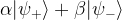
Let us now apply this idea to the problem of measuring one of the operators X_v. This operator is a tensor product of four $\sigma_x$ operators, i.e. inversion operators. Therefore a controlled-X_v circuit is nothing but a sequence of controlled inversions, i.e. CNOT gates. Thus we can measure a vertex operator using the following circuit.

Here the four qubits at the bottom correspond to the four edges meeting the vertex v. So we need one ancilla qubit for doing the measurement, and we need to be able to combine it in gates with all the four qubits sitting on the edges meeting v. For the physical implementation, the easiest approach is to place this additional qubit called measurement qubit in the vertex itself, in contrast to the data qubits that we have already placed on the edges. So we add one data qubit to each vertex.

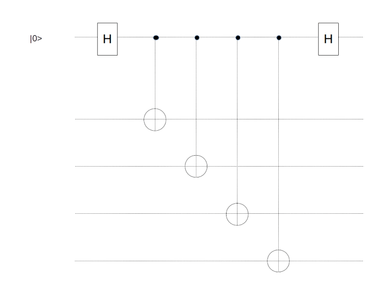
A circuit along the same lines can be constructed to measure Z_f for a face f. Using that $H \sigma_x H = \sigma_z$ , we can construct such a circuit as follows. In the first time step, apply a Hadamard to both the ancilla and all target qubits. Then apply CNOT operators to all target qubits, controlled by the ancilla, and then apply Hadamard operators again. Now, it is well known that conjugating the CNOT with Hadamard gates switches the roles of target qubits and control qubits. This gives us the circuit displayed below.

Again, for each face f, we need an ancilla qubit to measure Z_f. This qubit will have to interact with all data qubits on the edges bounding this face, so it is easiest to position it in the center of that face.

Overall, we have now added F + V measurement qubits to our original E data qubits. Now the Euler characteristic of the torus is zero, and therefore F + V = E, showing that this procedure actually doubles the number of physical qubits.

We have now arrived at a description of the toric code (and its cousin the surface code) that one can often find as a definition in the literature but which somehow obscures the relation to the surface topology a bit.

We start with a lattice L with E edges and identify opposite borders
On each vertex, we place a data qubit
On each face, we place a measurement qubit called a Z-qubit
On each vertex, we place a measurement qubit called an X-qubit
To each X-qubit, we associate the operator that acts as a bit flip on the four data qubits next to the measurement qubit
To each Z-qubit, we associate the operator that acts a a phase flip on the four data qubits next to the measurement qubit

Thus every data qubit is acted on by four operators, the two Z-operators corresponding to the adjacent faces and the two X-operators corresponding to the adjacent vertices. The additional measurement qubits – indicated by white circles in contrast to the dark circles being the data qubits – are shown below.

For one face and one vertex, we have indicated the associated operators X_v and Z_f by adding letters X and Z to show how these operators act on the nearby data qubits. This is the graphical representation typically used in the literature (like [3]). Note that some authors use different conventions and associate Z-operators with faces and X-operators with vertices, but this is of course completely equivalent due to the duality relations between a lattice and a dual lattice.

This completes our short introduction to toric codes. In the next post in my series on quantum error correction, we will pass on to a planar geometry which turns the toric code into a surface code.

References

1 A. Kitaev, Fault-tolerant quantum computation by anyons, arXiv:quant-ph/9707021
2. H. Bombin, An introduction to topological quantum codes, in Quantum error correction, edited by D.A. Lidar and T.A. Brun, Cambridge University Press, New York, 2013, available as arXiv:quant-ph/1311.0277
3. A.G. Fowler, M. Mariantoni, J.M. Martinis, A.N. Cleland, Surface codes: Towards practical large-scale quantum computation, arXiv:1208.0928v2

Kubernetes – an overview

Docker containers are nice and offer a very lean and structured way to package and deploy applications. However, if you really want to run large scale containerized applications, you need more – you need to deploy, orchestrate and manager all your containers in a highly customizable and automated way. In other words, you need a container management platform like Kubernetes.

What is a container management platform?

Imagine you have a nice, modern application based on microservices, and you have decided to deploy each microservice into a separate container. Thus your entire application deployment will consist of a relatively large number, maybe more than hundred, individual containers. Each of these containers needs to be deployed, configured and monitored. You need to make sure that if a container goes down, it is restarted and traffic is diverted to a second instance. You need to distribute your load evenly. You need to figure out which container should run on which virtual or physical machine. When you upgrade or deploy, you need to take dependencies into account. If traffic reaches a certain threshold, you would like to scale, either vertically or horizontally. And so forth…

Thus managing a large number of containers in a production-grade environment requires quite some effort. It would be nice to have a platform that is able to

Offer loadbalancing, so that incoming traffic is automatically routed to several instances of a service
Easily set up container-level networks
Scale out automatically if load increases
Monitor running services and restart them if needed
Distribute containers evenly across all nodes in your network
Spin up new nodes or shut down nodes depending on the traffic
Manage your volumes and storage
Offer mechanisms to upgrade your application and the platform and / or rollback upgrades

In other words, you need a container management platform. In this post – and in a few following posts – I will focus on Kubernetes, which is emerging as a de facto standard for container management platforms. Kubernetes is now the underlying platform for industry grade products like RedHat OpenShift or Rancher, but can of course be used stand-alone as well. In addition, all major cloud providers like Amazon (EKS), Google (GKE), Azure (AKS) and IBM ( IBM Cloud Kubernetes Service) offer Kubernetes as a service on their respective platforms.

Basic Kubernetes concepts

When you first get in touch with the world of Kubernetes, the terminology can be a bit daunting – there are pods, clusters, services, containers, namespaces, deployments, and many other terms that will be thrown at you. Time to explain some of the basic concepts very high level – we will get in closer contact with most of them over the next few posts.

The first object we need to understand is a Kubernetes node. Essentially, a node is a compute ressource, i.e. some sort of physical or virtual host on which Kubernetes can run things. In a Kubernetes cluster, there are two types of nodes. A master node is a node on which the Kubernetes components itself are running. A worker node is a node on which application workloads are running.

On each worker node, Kubernetes will start several agents, for instance the kubelet which is the primary agent responsible for controlling a node. In addition to the agent, there are of course the application workloads. One might suspect that these workloads are managed on a container basis, however, this is not quite the case. Instead, Kubernetes groups containers into objects called pods. A pod is the smallest unit handled by Kubernetes. It encompasses one or more containers that share resources like storage volumes, network namespaces and the same lifecycle. It is quite common to see pods with only one application container, but one might also decide to put, for instance, a microservice and a database into one pod. In this case, when the pod is started, both containers (the container containing the microservice and the container containing the database) are brought up on the same node, can see each other in the network under “localhost” and can access the same volumes. In a certain sense, a pod is therefore a sort of logical host on which our application containers run. Kubernets assigns IP addresses to pods, and applications running in different pods need to use these IP addresses to communicate via the network.

When a user asks Kubernetes to run a pod, a Kubernetes component called the scheduler identifies a node on which the pod is then brought up. If the pod dies and needs to be restarted, it might be that the pod is restarted on a different node. The same applies if the node goes down, in this case Kubernetes will restart pods running on this container on a different node. There are also other situations in which a pod can be migrated from one node to a different node, for instance for the purpose of scaling. Thus, a pod is a volatile entity, and an application needs to be prepared for this.

Pods themselves are relatively dumb objects. A large part of the logic to handle pods is located in componentes called controllers. As the name suggests, these are components that control and manage pods. There are, for instance, special controllers that are able to autoscale the number of pods or to run a certain number of instances of the same pod – called replicas. In general, pods are not started directly by a Kubernetes user, but controllers are defined that manage the pods life cycle.

In Kubernetes, a volume is also defined in the context of a pod. When the pod ceases to exist, so does the volume. However, a volume can of course be backed by persistent storage, in which case the data on the volume will outlive the pod. On AWS, we could for instance mount an EBS volume as a Kubernetes volume, in which case the data will persist even if we delete the pod, or we could use local storage, in which case the data will be lost when either the pod or the host on which the pod is running (an AWS virtual machine) is terminated.

There are many other objects that are important in Kubernetes that we have not yet discussed – networks, services, policies, secrets and so forth. This post is the first in a series which will cover most of these topics in detail. My current plans are to discuss

Creating and maintaining Kubernetes clusters using Python (part I, part II)
Working with pods and deployments
Exposing services to the outside world – services and load balancers
A deep dive into Kubernetes networking
Ingress rules and Ingress controllers
Kubernetes storage concepts
Stateful sets
Custom resource definitions
Custom controllers

Thus, in the next post, we will learn how to set up and configure AWS EKS to see some pods in action (I will start with EKS for the time being, but also cover other platforms like DigitalOcean later on).

Factoring integers on a quantum computer with Qiskit

After all the work done in the previous posts, we are now ready to actually implement Shor’s factoring algorithm on a real quantum computer, using once more IBMs Q Experience and the Qiskit framework.

First, recall that Shor’s algorithm is designed to factor an integer M, with the restriction that M is supposed to be odd and not a prime power. Thus the smallest meaningful value of M is M=15. Of course this is a toy example, but we will see that even this toy example can be challenging on the available hardware. Actually, 15 is also the number that was factored in the first implementation of Shor’s algorithm on a real quantum computer which used an NMR based device and was done in 2001 – see [1].

The quantum part of the algorithm is designed to find the period r of a chosen number a modulo M. There are several choices of a that are possible, the only condition we need is that a and M are co-prime. In this post, we follow the choice in [1] and use a = 11 and a = 7. As in [1] (and all other similar papers I am aware of, see also the discussion in this paper by Smolin, Smith which later appeared in Nature) we will also rely on prior knowledge of the result to build up our circuits, so we are actually cheating – this is not really an application of Shor’s algorithm, but merely a confirmation of a known factoring.

Of course, it is easy to compute the period directly in our case. The period of a = 11 is two, and the period of a = 7 is four. A smaller period means a simpler circuit, and therefore we start with the case a = 11. Let us see whether we can confirm the period.

The easy case – a = 11

For our tests, we will use the description of Shor’s algorithm in terms of the quantum phase estimation procedure. Thus we have a primary register that we initialize in the state $|1\rangle$ and to which we apply a sequence of controlled multiplications by powers of a, and a working register, in which we do a quantum Fourier transform in the second step. The primary register needs to hold M=15, so we need four qubits there. For the working register, we use three qubits, which is the smallest possible choice, to keep the number of gates small.

The first step of our algorithm is controlled multiplication by a. However, this is greatly simplified by the fact that we apply this to exactly one state that we know upfront – the initial state $1 \rangle$ . Thus we only need to implement a unitary transformation which conditionally maps the state $|1 \rangle$ to the state $|a = 11 \rangle$ . In binary notation, eleven is 1011, and we therefore simply need to conditionally flip qubits 3 and 1. We also need a Pauli X gate in the primary register to build the initial state $|1 \rangle$ from the fiducial state $|0\rangle$ and Hadamard gates in the working register to create the initial superposition. Thus the first part of our circuit looks as follows.

What about higher powers of a? This is easy – we know that a² is equal to one modulo M, and therefore the multiplication by a² modulo M is simply the identity transformation. The same is true for all even powers and so we are already done with the first part of our circuit – this is why we call the case a = 11 the easy case. The only thing that is left is to add the quantum Fourier transformation and a measurement to the working register. This gives us the following circuit (which can obviously be simplified, more on this later).

Now we can run this on a simulator. Before we do this, let us try to understand what we expect. We know that after measuring the working register, the value that we obtain is a multiple of 2³ / r = 8 / 2 = 4. Thus we expect to see peaks at 0 and four (binary 100). And this is actually what we get – the following histogram shows the output of an execution on the local QASM simulator integrated into Qiskit.

This is nice, our circuit seems to work correctly. So let us proceed and try this on real hardware. Before we do so, however, let us simplify our circuit a bit to reduce the number of gates needed and thus the noise level. First, we skip the final swap gates in the QFT circuit – this will change our expected output from 100 to 001, but we can keep track of this manually when setting up the measurement. Next, we have two Hadamard gates on w[2] that cancel and that we can therefore remove. And the Pauli X gate on p[0] is never really used and can be dropped. After these changes, we obtain the following circuit.

We can run this on the IBMQ hardware. As we require seven qubits in total, we need to do this on the 14 qubit model ibmq_16_melbourne. Here are the results of a test run, again as a histogram.

We see the expected peaks at 000 and 100, but also see some significant noise that is of course not present in the simulation. However, the probabilities to measure one of the theoretically expected values is still roughly twice as high as the probability of any of the other values.

The hard case – a = 7

Having mastered the case a = 11, let us now turn to the case a = 7. The only change that we need to make is the circuit acting on the primary register. In the first part of the circuit, we can again make use of the fact that we only have to deal with one possible input, namely the initial state $|1 \rangle$ . The conditional multiplication by a maps this to $|7\rangle$ , and we can again implement this by two conditional bit flips, i.e. two CNOT gates.

The second part, the conditional multiplication by a² = 4 modulo M, requires a bit more gates. On a bit level, multiplication by four is a bit shift by two bits to the left. We can realize this as a sequence of two conditional swap gates, swapping the bits zero and two and the bits one and three. A conditional swap gate can be implemented by three CNOT gates, or, in QASM syntax,

gate cswap a,b,c
{
  cx c,b;
  ccx a,b,c;
  cx c,b;
}

We can also make a few simplifications by replacing CNOT gates with fixed values of the control qubit by either an inversion or the identity. We arrive at the following circuit.

This is already considerably more complex than for the case a = 11. When we add the QFT circuit and the measurements, we end up with the following circuit.

Now the period is four. Thus we expect peaks at all multiples of two, i.e. at all even values. And this is actually what we get when we run this on a simulator.

Now let us again see how we can optimize this circuit before trying it on real hardware. Again, there are a few additional simplifications that we can make to reduce the noise level. On w[2], we have a double Hadamard gate that we can remove. We can again dispose of the final swap gates and move the swap operation into the measurement. The last CNOT between p[1] and p[3] can be dropped as it does not affect the outcome. The same is true for the last CNOT between p[0] and p[2]. Thus we finally arrive at the following circuit.

And here is the result of running this on the 16 qubit IBM device.

Surprisingly, the noise level is not significantly worse than for the version with a = 11, even though we have a few more gates. We can clearly see that the probabilities to measure even values are significantly higher than the probabilities to measure odd values, corresponding to the period four.

So what did we learn from all this? First, our example was of course a toy model – we did code the circuit based on knowledge on the period and hard-coded the value of a. However, our example demonstrates the basic techniques to build circuits for the more general case. In real application, we could, given a number M, first determine a suitable value for a. The conditional multiplication by a is then acting as a permutation on the computational basis and can therefore be implemented by a sequence of (conditional) swap gates. The same is true for higher powers of a. So in theory, we have all the ingredients that we need to implement more general versions of the algorithm.

In practice, however, we will quickly reach a point where the number of gates exceeds the limit that we can reasonable implement given the current level of noise. So real applications of the algorithm in number ranges that are not tractable for classical digital computers will require advanced error correction mechanisms and significantly reduced noise levels. Still, it is nice (and fun) to see a toy version of the famous algorithm in action on a real device.

If you want to run the examples yourself, you can use my notebooks for the case a=11 and a=7.

References

1. L. Vandersypen, M. Steffen, G. Breyta, C. Yannoni, M. Sherwood, I. Chuang, Experimental realization of Shor’s quantum factoring algorithm using nuclear magnetic resonance, Nature Vol. 414, (December 2001)
2. P. Shor, Polynomial-Time Algorithms for Prime Factorization and Discrete Logarithms on a Quantum Computer, SIAM J.Sci.Statist.Comput. Vol. 26 Issue 5 (1997), pp 1484–1509, available as arXiv:quant-ph/9508027v2
3. R. Cleve, A. Ekert, C. Macchiavello, M. Mosca, Quantum Algorithms revisited, arXiv:9708016
4. A. Kitaev, Quantum measurements and the Abelian Stabilizer Problem, arXiv:quant-ph/9511026
5. J. Smolin, G. Smith, A. Vargo, Pretending to factor large numbers on a quantum computer, arXiv:1301.7007 [quant-ph]

Quantum phase estimation – the quantum algorithm Swiss army knife

When you are faced with a problem in linear algebra and have absolutely no idea what to do, an eigenvalue decomposition is the one thing that you would typically try first. In the world of quantum algorithms, the situation is similar – finding the eigenvalues of a matrix is a central building block of many quantum algorithm. The most important approach to finding the eigenvalues is called the quantum phase estimation algorithm.

The quantum phase estimation algorithm

In its most basic form, the quantum phase algorithm is used to find an eigenvalue of a unitary matrix assuming that we know an eigenvector (we will see later that this is in fact not necessarily needed for useful applications). So let us assume that we are given a unitary matrix U, implemented as a quantum circuit, and a quantum state $|\psi \rangle$ which is an eigenvector of U. As U is unitary, all eigenvalues are on the complex unit circle, and therefore the eigenvalue equation is

$U |\psi \rangle = e^{2\pi i \varphi} |\psi \rangle$

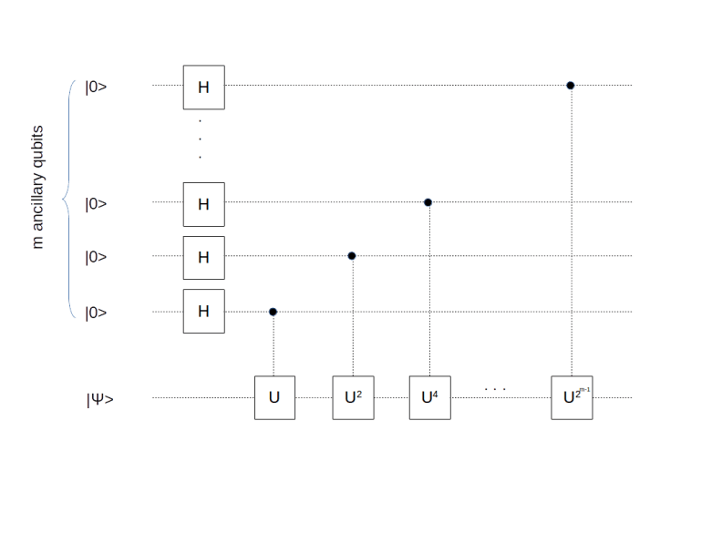
for some number $\varphi$ between zero and one. The quantum phase estimation is designed to determine (or at least approximate) the number $\varphi$ , i.e. the phase of the eigenvalue (hence the name).

The algorithm consists of two parts. Both parts operate on an ancillary working register and a register that we call the primary register. Let n denote the number of qubits in the primary register and m denote the number of qubits in the working register. We assume that the initial state in the primary register is the state $|\psi \rangle$ . The first step of the algorithm is to prepare the system in the state

$\frac{1}{\sqrt{2^m}} \sum_{k=0}^{2^m - 1} |k \rangle U^k |\psi \rangle$

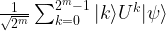
How can we prepare this state? Given a state $|k \rangle$ , with binary digits k_i, we can of course write U^k as

$U^k = \prod_i \big[ U^{2^i} \big]^{k_i}$

In other words, U^k is a sequence of conditional gates U^2ⁱ, conditioned on the i-th bit of k. Together with the usual approach to prepare an equal superposition of all $|k \rangle$ by using Hadamard gates, this argument shows that the desired state can be prepared by the following quantum circuit.

So far we have not yet used that the initial state $|\psi \rangle$ is an eigenstate. Let us do this now. We know that a power of U will act on $|\psi \rangle$ as multiplication by the corresponding power of the eigenvalue, hence

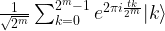
$\frac{1}{\sqrt{2^m}} \sum_{k=0}^{2^m - 1} |k \rangle U^k |\psi \rangle = \frac{1}{\sqrt{2^m}} \big[\sum_{k=0}^{2^m - 1} e^{2\pi i \varphi k} |k \rangle \big] \otimes |\psi \rangle$

This is interesting – our state turns out to be a product state (as the multiplication by a scalar can be pulled through the tensor product). To understand the first part of the product (i.e. the resulting state in the working register) in more detail, let us assume for a moment that the phase $\varphi$ is an exact multiple of 2^-m, i.e. that

$\varphi = \frac{t}{2^m}$

for some integer t. Then the state in the working register is

$\frac{1}{\sqrt{2^m}} \sum_{k=0}^{2^m - 1} e^{2\pi i \frac{tk}{2^m}} |k \rangle$

But this is simply the inverse quantum Fourier transform applied to the state $|t \rangle$ ! So we can obtain t and therefore $\varphi$ by applying a quantum Fourier transform to the state in the working register and doing a measurement. This is the quantum phase estimation algorithm.

In most cases, the phase will of course not be an exact multiple of t / 2^m. However, with a bit more work (see for instance arXiv:quant-ph/9708016 or my own notes) one can see that the our result is still approximately true, i.e. if we run this algorithm, measure the value in the working register and divide by 2^m, we get a good approximation to the actual phase $\varphi$ . The precision of the estimation depends on the number of qubits m that we have in our working register. The following diagram demonstrates this for a specific example for two different values of m.

The x-axis shows the absolute deviation from the true value, the y-axis shows the probability for this deviation. The upper image corresponds to m=3. We see that there is a peak around zero, but still a substantial probability to have a significant error. The lower diagram shows the outcome for m=8. Here we see that the peak is very sharp, and so we obtain a very good approximation with high probability.

Shor’s algorithm as an instance of quantum phase estimation

Most of the time, the quantum phase estimation algorithm is used as a subroutine in a more general algorithm. A prominent example is Shor’s algorithm which – as we will now see – can be expressed as an application of the quantum phase estimation.

Recall that the quantum part of Shor’s algorithm is concerned with finding the period of a number a modulo M, where M is some large integer that we want to factor. Here we assume that a is a unit modulo M so that one of its powers is one. As a is a unit, the mapping

$U \colon |x \rangle \mapsto |ax \mod M\rangle$

is a unitary transformation U for x < M (which we can extend by the identity to a unitary transformation of the full Hilbert space). If r denotes the period of U, then clearly the fact that a^r = 1 modulo M implies that U^r = 1. Thus all eigenvalues of U are r-th roots of unity. In other words, if an eigenvalue has phase $\varphi$ , then $\varphi r$ is an integer. We can therefore use the phase estimation algorithm to obtain the period r.

There is one twist, however. To be able to apply the phase estimation algorithm, we need an eigenvector as an initial state, and it is far from clear how to prepare this. Fortunately, a deeper analysis (again see arXiv:quant-ph/9708016 or my own notes for all the details of this) shows that the state $|1 \rangle$ is a sum of eigenstates. Running the algorithm on this state will – by linearity – produce a state which is a superposition of states corresponds to different multiples of 2^m / r, and performing the measurement will choose one of these multiples. As in Shor’s original version of the algorithm, we can then use a continued fraction expansion to obtain the unknown period r. Thus, the following algorithm can be used to determine the period r.

Prepare a primary register in the state $|1 \rangle$
Apply the circuit shown above
Apply a quantum Fourier transform to the working register
Perform a measurement of the working register and call the result s – this will be close to a multiple of 2^m / r
Perform a continued fraction expansion to find the period r as in Shor’s original version of the algorithm

At the first glance, it looks as if we had found an alternative period finding algorithm, but if you actually draw up the circuit that realizes this algorithm, you will find – again see the references cited before – that this is not true, in fact the resulting circuit will be almost identical to the circuit for Shor’s version of the algorithm. Thus we have not found a new algorithm, but have found a different description of the same algorithm – period finding can be described as an instance of the phase estimation algorithm.

More applications

Of course factoring integers is not the only possible application of the quantum phase estimation. An obvious application is finding eigenvalues of Hamiltonians, i.e. energy eigenvalues – and in particular ground state energies – of physical systems. We have already touched on this possible application in a previous post on the quantum variational eigensolver.

Another application is based on the observation that if we start the algorithm with a superposition of eigenvectors, the measurement at the end of the algorithm will not only select an eigenvalue, but also an eigenvector. Thus we can use the algorithm to decompose a state into a superposition of eigenvectors. This can be used to solve linear equations of the form Ax = b for a given matrix A. In fact, if we can diagonalize A, then solving this equation becomes equivalent to division. Implementing this as a quantum algorithm is not as simple and straightforward as this description might suggest, as the division is a non-unitary operation, but it turns out that it can be approximated by a unitary transformation. The resulting algorithm is called the HHL-algorithm after its inventors Harrow, Hassidim and Lloyd, and has been published in this paper on the arxiv.

The HHL algorithm does not guarantee a quantum advantage for every matrix A, as it relies on a way to efficiently calculate the corresponding time evolution operators e^iAt. However, if for instance A is sparse and has low condition number (ratio between eigenvalues), the algorithm provides an exponential speedup over the best classical algorithms. An important application is deep machine learning, where efficient matrix inversion plays an important role – see for instance this paper by Zhao, Pozas-Kerstjens, Rebentrost, and Witte, as well as the corresponding source code. The details of the HHL algorithm are far from being trivial, and we will leave a more in-depth discussion to a future post.