When I tried to learn about neuronal networks first, I did what probably most of us would do – I started to look for tutorials, blogs etc. on the web and was surprised by the vast amount of resources that I found. Almost every blog or webpage about neuronal networks has a section on training a simple neuronal network, maybe on the MNIST data set, using a framework like TensorFlow, Theano or MXNET. When you follow such a tutorial, a network is presented as a collection of units and weights. You see how the output of the network is calculated and then an error function – sometimes least squares, sometimes something else – is presented. Often, a regulation term is applied, and then you are being told that the automatic gradient calculation features of the framework will do the gradient descent algorithm for you and you just have to decide on an optimizer and run the network and enjoy the results.
Sooner or later, however, you will maybe start to ask a few questions. Why that particular choice of the loss function? Where does the regulator come from? What is a good initial value for the weights and why? Where does the sigmoid function come from? And many, many other questions….
If you then decide to dig deeper, using one of the many excellent textbooks or even try to read some of the original research papers (and some are actually quite readable), you will very soon be confronted with terms like entropy, maximum likelihood, posterior distribution, Gaussian mixtures and so on, and you will realize that the mathematics of neuronal networks has a strong overlap with mathematical statistics. But why? Why is that a good language to discuss neuronal networks, and why should you take the time to refresh your statistics knowledge if you really want to understand neuronal networks? In this post, I will try to argue that statistical inference comes up very naturally when you try to study neuronal networks.
Many neuronal networks are designed to excel at classification tasks. As an example, suppose you wanted to design and train a neuronal network that, given data about an animal, classifies the animal as either a bird or some other animal (called a “non-bird” for convenience). So our starting point is a set modelling all possible objects that could be presented to the network. How exactly we model this set is not so important, more important is that in general, the network will not have access to all the data about the animal, but only to certain attributes of elements in the set called features. So there could be a feature which we call X1 and which is defined as

taking values in 

taking values in the reals and so forth. More generally, we assume that on the set of all possible objects, we have certain functions Xi taking values in, say, the real numbers. Based on these numbers, the network will then try to take a decision whether a given animal is a bird or not. Thus we do not have to deal directly with our space of objects, but use the functions Xi as primary objects.
If the network had a chance to look at every possible animal, this would be easy, even though it would cost a lot memory – it could simply remember all possible combinations of features and for each feature, store the correct answer. In reality however, this does not work. Instead, we have access to a small subset of the data – a sample – for which we can evaluate the Xi. Based on this subset, we then have to derive a model which gives the right answer in as many cases as possible. Thus we try to make a statement about the full space of things that could be presented to our network for classification based on a small sample.
This is where probabilities come into play very naturally. We need to assume that our sample has been chosen randomly, but still we need to make assertions about the full set. This is exactly what inferential statistics is doing. The fact that our sample is chosen randomly turns our Xi into random variables. Similarly, the variable

taking values in
Apart from the fact that we have to derive information on the full population based on a sample, there is another reason why probabilities appear naturally in the theory of machine learning. In many cases, the available input – being a reduction of the full set of data – is not sufficient to classify the sample with full certainty. To see this, let us go back to our examples. How would you derive the property “bird” from the given data “can fly” and “length”? Not all animals than can fly are birds – and not all birds can fly. So we have to try to distinguish for instance a butterfly from a hummingbird based on the length. The smallest hummingbird – a bee hummingbird – is about 5 cm in length. The largest known butterfly – the Queen’s Alexandra birdwing – can be as long as 8 cm (both informations taken from Wikipedia). Thus our data is not sufficient to clearly distinguish butterflies and birds in all cases!
However, very small birds and very large butterflies have one thing in common – they are rare. So chances are that a given animal that can fly and is larger than 5 cm is actually a bird (yes, I know, there are bats….). In other words, if again Y denotes the variable which is 1 on birds and 0 on all other animals, we can in general not hope that Y is a function of the Xi, but we can hope that given some values of the Xi, the probability 

with some unknown function f. In a Bayesian interpretation of probability, the certainty with which can say “this animal is a bird” is a function of the values xi of the observable variables Xi.
With these considerations, we now arrive at the following mathematical model for what a classification algorithm is about. We are given a probability space 

where 

This model sounds a bit abstract, but many feed forward neuronal networks can be described with this or similar models. And we can now apply the full machinery of mathematical statistics – we can calculate cross entropies and maximum likelihood, we can analyse converge and variance, we can apply the framework of Bayesian statistics and Monte Carlo methods. This is the reason why statistics is so essential when it comes to describing and analyzing neuronal networks. So on the next rainy Sunday afternoon, you might want to grab a steaming hot cup of coffee, head towards your arm chair and spent some time with one of the many good exposures on this topic, like chapter IV in MacKays book on Machine Learning, or Bishops “Pattern recognition and machine learning” or chapter 3 of the deep learning book by Goodfellow, Bengio and Courville.

 on some state space X (most often this will be a real euclidian space on which you can do floating point arithmetic). You might want to imagine the state space as describing possible states of a physical system, like spin configurations in a ferromagnetic medium similar to what we looked at in my post on the
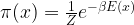
 for a single point in the state space intractable.

 .
. 

 . We now calculate
  according to the formula above. We then accept the proposal with probability
  . If the proposal is accepted, we set xn+1 = y, otherwise we set xn+1 = xn, i.e. we stay where we are.

 with probability one. This is very similar to a random search for a global maximum – we start at some point x, choose a candidate for a point with higher value of
  with a non-zero probability. This allows the algorithm to escape a local maximum much better. Intuitively, the algorithm will still try to spend more time in regions with large values of
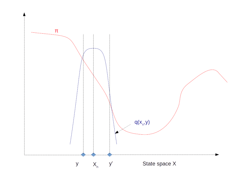
 and
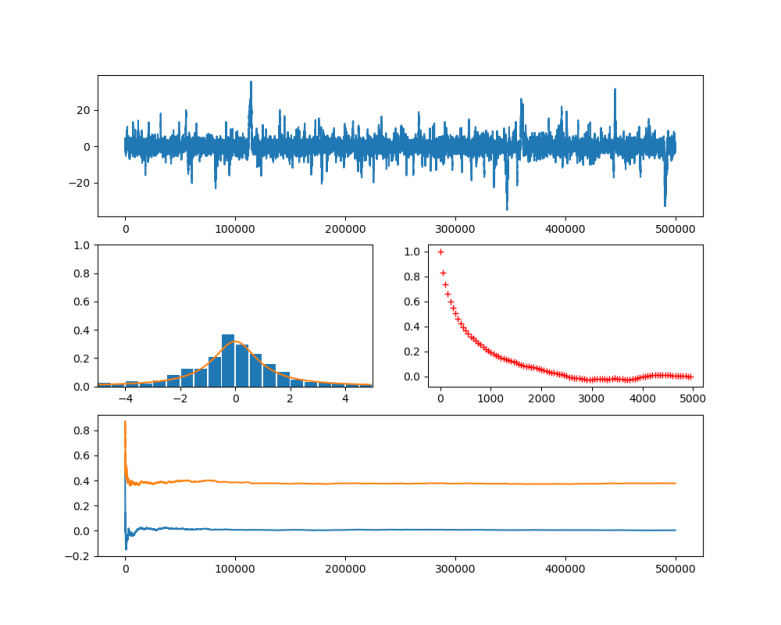
and  ) approximated using the partial sums develops over time. We see that even though we still have huge spikes, the integral remains comparatively stable and converges already after a few thousand iterations. Even if we run the simulation only for 1000 steps, we already get close to the actual values zero (for
  (for
(for 
 and
and  are the standard deviations of X and Y. In our case, given a lag, i.e. a number l less than the length of the chain, we can form two samples, one consisting of the points
  and the second one consisting of the points of the shifted series
  . The autocorrelation with lag l is then defined to be the correlation coefficient between these two series. In the diagram, we can see how the autocorrelation depends on the lag. We see that for a large lag, the autocorrelation becomes small, supporting our intuition that the series and the shifted series become independent. However, if we execute several simulation runs, we will also find that in some cases, the convergence of the autocorrelation is very slow, so care needs to be taken when trying to obtain a nearly independent sample from the chain.
  , we can use the conditional probability given either x1 or x2 as a proposal distribution. Thus, we first fix x2, and draw a new value for x1 from the conditional probability for x1 given the current value of x2. Then we move to this new coordinate, fix x1, draw from the conditional distribution of x2 given x1 and set the new value of x2 accordingly. It can be shown (see for example