May 2018 – LeftAsExercise

Recurrent and ergodic Markov chains

Today, we will look in more detail into convergence of Markov chains – what does it actually mean and how can we tell, given the transition matrix of a Markov chain on a finite state space, whether it actually converges.

So suppose that we are given a Markov chain on a finite state space, with transition probabilities described by a matrix K as in the previous post on this topic.

We have seen that the distribution of X_n is given by $\mu K^n$ where $\mu$ is the initial distribution. So if Kⁿ converges, we can expect the distribution of X_n to converge as well. If there is a matrix $K^\infty$ such that

$\lim_{n \rightarrow \infty} K^n = K^\infty$

then of course

$K^\infty K = (\lim_{n \rightarrow \infty} K^n) K = \lim_{n \rightarrow \infty} K^{n+1} = K^\infty$

In other words, each row $\pi$ of $K^\infty$ will have the property that $\pi K = \pi$ . Interpreting K as transition probabilities, this implies that if the distribution of X_n is $\pi$ , the distribution of X_n+1 will again be $\pi$ . Any distribution, described by a row vector $\pi$ with row sum 1, for which this holds is called an invariant distribution and traditionally denoted by $\pi$ . In other words, invariant distributions correspond to eigenvectors of the transposed matrix K^T with eigenvalue 1, and our argument has shown that if $K^n$ converges to $K^\infty$ , then every row of $K^\infty$ will be an invariant distribution.

So convergence implies the existence of an invariant distribution. Let us next try to understand whether this invariant distribution is unique. There are obvious examples where this is not the case, the most trivial one being the unit matrix

$K = \begin{pmatrix} 1 & 0 \\ 0 & 1 \end{pmatrix}$

Obviously $K^n = K$ and the chain converges, but every vector with row sum one is an invariant distribution. This chain is too rigid, because in whatever state we start, we will stay in this state forever. It turns out that in order to ensure uniquess of an invariant distribution, we need a certain property that makes sure that the states can move around freely which is called irreducibility.

Intuitively, we say that a Markov chain is irreducible if any state can be reached from any other state in finitely many steps. For a finite state space, this is rather easy to formalize. A finite Markov chain is called irreducible if, given two states i and j, we can find some power n such that $K^n_{ij} > 0$ . In other words, given a row index i and a column index j, we can find a power n such that the element of Kⁿ at (i,j) is not zero. It turns out that if a chain is not irreducible, we can split the state space into smaller areas that the chain – once it has entered one of them – does not leave again and on which it is irreducible. So irreducible Markov chains are the buildings blocks of more general Markov chains, and the study of many properties of Markov chains can be reduced to the irreducible case.

Now let us assume that our chain is in fact irreducible. What else do we have to ask for to make sure that it converges? Again, let us as look at an obvious example.

$K = \begin{pmatrix} 0 & 1 \\ 1 & 0 \end{pmatrix}$

All even powers of this matrix are the unit matrix and all odd powers are K itself, so the Markov chain described by this transition matrix is clearly irreducible. However, there is still something wrong. If, for instance, we are in state 1 at the time t, then the probability to still be in state 1 at time t+1 is zero. Thus we are actually forced to move to state 2. In a certain sense, there is still an additional constraint on the the behaviour of the chain – the state space can be split in two pieces and we cycle through these pieces with every step. Such a chain is called periodic. If a chain is periodic, it is again obvious that we can think of it as two different chains, one chain given by the random variables X₀, X₂,… at even times and the other chain given by the random variables X₁, X₃, … at odd times. Thus again, there is a way to split the chain into parts.

So let us now focus on chains that are irreducible and aperiodic. Can we tell whether the chain converges? The answer is surprisingly simple and one of the most powerful results in the theory or Markov chains: every finite Markov chain which is irreducible and aperiodic converges. Thus once we have verified aperiodicity and irreducibility, we can be sure that the limit $K^\infty$ exists. We can say even more – we have seen that the rows of the limit are invariant distributions for K. However, one can show that an irreducible Markov chain can only have one invariant distribution. Thus we can conclude that all rows of the matrix $K^\infty$ are identical. In fact, they are all equal to the (unique) invariant distribution that again corresponds to an eigenvector of K^T with eigenvalue one.

This gives us two different approaches to calculating the invariant distribution and the limit $K^\infty$ . First, we can form high powers Kⁿ to approximate the limit $K^\infty$ . Or, alternatively, we can search for eigenvectors of the transposed matrix K^T with eigenvalue 1 using one of the known algorithms to calculate eigenvectors and eigenvalues.

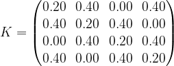
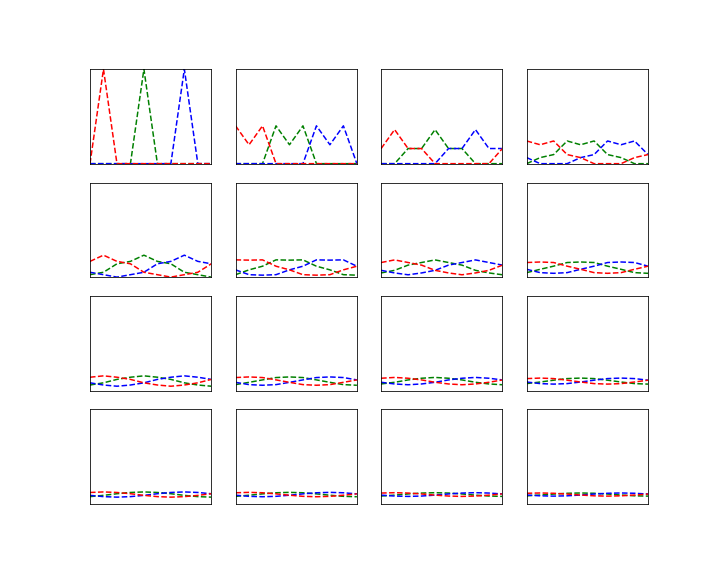
Let us do this for the example of the random walk on a circle that we have studied earlier. For simplicity, we will use N = 4 this time. The transition matrix with p = 0.8 is

$K = \begin{pmatrix} 0.20 & 0.40 & 0.00 & 0.40 \\ 0.40 & 0.20 & 0.40 & 0.00 \\ 0.00 & 0.40 & 0.20 & 0.40 \\ 0.40 & 0.00 & 0.40 & 0.20 \\ \end{pmatrix}$

We can then easily implement both approaches in Python using the numpy library.

Sorry, something went wrong. Reload?

Sorry, we cannot display this file.

Sorry, this file is invalid so it cannot be displayed.

view raw TransitionMatrixMarkovChain.ipynb hosted with ❤ by GitHub

So we see that the approach to take the eigenvalues and eigenvectors gives us – in this case – the exact result (and a direct computation confirms that this is really an eigenvector), whereas the matrix power with n=20 gives a decent approximation. Both results confirm what we have observed visually in the last post – the distribution converges, and it does in fact converge to the uniform distribution. So roughly speaking, after sufficiently many steps, we end up everyhwere in the state space with equal probability.

So far, we have only discussed the case of a finite state space. In the general case, the situation is more complicated. First, we need a better definition of irreducibility, as on a general state space, the probability measure of a single point tends to be zero. It turns out that the solution is to define irreducibility with respect to a measure on the state space, which is called $\psi$ -irreducibility. Once we have that, we find two potential behaviours that do not show up in the finite case.

First, it might happen that even though the chain is irreducible, it does not properly cycle through the state space and revisits every point with finite probability, but – intuitively speaking – heads off to infinity. Such a chain is called transient and does not converge.

Second, even if the chain is not transient, we might be able to find an invariant distribution (a measure in this case), but this measure might not be a probability distribution as it is not finite. Chains with this property are called null recurrent.

And finally, the concept of converge needs to be made more precise, and it turns out to have a subtle dependency on the starting point which can be fixed by assuming so called Harris recurrence. But all this can be done and delivers a very similar result – a convergence theorem for a large class of chains (in this case aperiodic Harris recurrent Markov chains). If you would like to get deeper into this and also see proofs for the claims made in this post and references, I invite you to take a look at my short introduction to Markov chains.

We close this post with one remark which, however, is of crucial importance for applications. Suppose we have a convergent Markov chain X_t, and a function f on the state space. If the X_t were independent and identically distributed, we could approximate the expectation value of f as

$\int_X f(x) dP = \lim_{N \rightarrow \infty} \frac{1}{N} \sum_{i=1}^N f(X_i)$

where dP is the (common) distribution of the X_t. For Markov chains, however, we know that the X_t are not independent – the whole point of having a Markov chain is that X_t+1 does actually depend on X_t. However, in our example above, we have seen that the dependency gets trivial for large t as in this example, all entries in the transition matrix become equal in the limit.

Of course this is a special case, but it turns out that even in general, the approximation of the expectation value by averages across the sample is still possible. Intuitively, this is not so surprising at all. If the distributions $K^n$ of the $X_n$ converge to some invariant measure $\pi$ , the $X_n$ will, for large n, be approximately identically distributed, namely according to $\pi$ . Moreover, heuristically we have for large n, m and a fixed starting point s:

$P(X_{n+m}=i, X_n=j) = K^m_{ji} K^n_{sj} \approx \pi_i \pi_j$

On the other hand, this product is again approximately the product

$\pi_i \pi_j \approx P(X_{n+m}=i) P(X_n=j)$

Thus, intuitively, X_n and X_m are almost independent if n and m are large, which makes us optimistic that the law of large numbers could actually hold.

In fact, if X_t converges (again I refer to my notes for a more precise definition of convergence in this case), it turns out that the law of large numbers remains valid if we integrate f with respect to the invariant distribution $\pi$ :

$\int_X f(x) d\pi = \lim_{N \rightarrow \infty} \frac{1}{N} \sum_{i=1}^N f(X_i)$

This is extremely useful in applications, where often the primary purpose is not so much to obtain a sample, but to approximate otherwise intractable integrals! Once we have found a Markov chain that converges to the invariant distribution $\pi$ , we can calculate integrals over $\pi$ by running a long Markov chain until converge and then taking the average value of the function that we want to integrate for a large number of subsequent points from this chain. In fact, this is how most applications work – and this is more or less what we also did when we applied Markov chains to the problem of calculating gradients in the PCD algorithm, where this chain is given by the state of the negative particles in subsequent iterations.

So given a distribution $\pi$ , we are now lead to the question how we can possibly find a Markov chain for which this distribution is invariant and which converges. The most general answer to this question is a class of algorithms known as Metropolis-Hastings algorithms which we study in the next post in this series.

Merkle trees

Suppose you are given a long file and wanted to use hashing to verify the integrity of the file. How would you do this in the most efficient way?

Of course, the first thing that might come to your mind is to simply take a hash of the entire file. This is very easy, but has one major disadvantage – if the file is damaged, there is no way to tell which part of the file has been damaged. If you use such a mechanism for instance to verify the integrity of a large download, you will have to go back and download the entire file again, which is very time consuming.

A smarter approach is to split the file into data blocks. You then calculate a hash for each data block to obtain a hash list. Finally, you could concatenate all the hashes into one large string and take the hash of that string. If a recipient of the file has access to only this top level hash, she could already verify the integrity of the file by repeating this procedure and comparing the top level hash with the hash created by the sender.

If that check fails, there is no need to re-transmit the entire file. Instead, the recipient could obtain a copy of the hash list itself and compare the hashes block by block until the faulty block is detected. This block can then be exchanged and the procedure can be repeated to verify that the replacement is valid. The bittorrent protocol uses this mechanism to detect inconsistencies in transferred files.

With a simple hash list like this, you would have to search the entire hash list in order to determine the faulty piece, requiring a time linear in the number of blocks. Searching can be improved greatly by organizing the hashes not into a list, but into a (binary) tree – and this data structure is called a hash tree or Merkle tree.

To illustrate the principle, suppose you wanted to build a hash tree for a file consisting of eight blocks, labeled 1 – 8.

You would then proceed as follows, as indicated in the image above. First, you compute the hash value for all blocks and assign them as values to the eight leaves of the tree. Then, you concatenate the values of leaves 1 and 2 and take the hash value of the result. This gives you the value for the parent node – called a in the picture above – of 1 and 2. You repeat the same procedure for the leaves 3 and 4, this gives you the value for the node b. Then you concatenate the values of a and b and take the hash value of the result, this gives you the value of the node c. Repeat this procedure for the right part of the tree and assign the result to node d. Finally, concatenate the values of node c and d and take the hash – this will be the value of the root node called the Merkle root. Thus, in a binary Merkle tree, the value of each node is defined to be the hash of the concatenation of the values of its two child nodes.

How is a Merkle tree realised in the bitcoin reference implementation? The currently relevant code is in consensus/merkle.cpp. This implementation is already optimized, the original implementation used to be in primitives/block.cpp and is still available on GitHub.

As the comments in the source code explain, at any level of the tree, the last node is added at the end again if needed to make sure that the number of nodes is even at each level – the algorithm that I have illustrated above only works if the number of leaves is a power of two. The actual implementation first builds a list of the leaves. It then goes through the list and for any two subsequent elements, it adds an element at the end which is the hash of the concatenation of these two elements. The last element is then the Merkle root that we are looking for.

Let us now see how a straightforward implementation looks like in Python.

Sorry, something went wrong. Reload?

Sorry, we cannot display this file.

Sorry, this file is invalid so it cannot be displayed.

view raw MerkleRoot.ipynb hosted with ❤ by GitHub

Most of the code should be self explaining, but a few remarks are in order. First, the hash function that we use could of course by any hash function, but, to be consistent with what bitcoin is doing, we use a double SHA256 hash. Then, byte ordering is again to be observed. The bitcoin reference client uses the method GetHash() on the involved transactions to populate the leaves, and we know that this is providing the transaction ID in little endian byte order. The entire calculation then proceeds in little endian byte order. The JSON output, however, display the transaction IDs in big endian order and the same holds for the Merkle root. Thus we need to reverse the byte order before we build the tree and, when comparing our result with the Merkle root which is part of the block, reverse the byte order again.

The actual calculation of the Merkle root uses a very straightforward approach – instead of maintaining one long list as the original bitcoin reference representation did, we represent the nodes at each level of the tree by a separate list and use recursion. This is probably a bit less efficient, but maybe easier to understand.

In order to test our implementation, we finally use the Python requests library to get a block in JSON format from blockchain.info using their REST API. We then build the leaves of the tree by walking through the list of transaction IDs in the block, build the Merkle root and compare the result to the value which is part of the JSON block structure. Nice to see that they match!

What happens if a client wants to verify that a given transaction is really included in a block without downloading the full block? In this case, it can ask the bitcoin server (either via the RPC call gettxoutproof or as part of the GETDATA network message) to provide a Merkle block, which is a serialized instance of CMerkleBlock. Essentially, a Merkle block consists of a block header plus a branch of the Merkle tree that is required to verify that a specific transaction is part of the block. This eliminates the need to transfer all transactions (which can be several thousand) while still allowing the client to check that a transaction is really included in a block.

This completes our short discussion of Merkle trees. We are now able to calculate the Merkle root for inclusion in a block header given the list of transactions that a block contains. To be able to mine a block, there is one more thing that we need to understand and that we will cover in the next post in this series – mining difficulty and the proof-of-work target.

Finite Markov chains

In this post, we will look in more detail into an important class of Markov chains – Markov chains on finite state spaces. Many of the subtleties that are present when studying Markov chains in general state spaces do not appear in the finite case, while most of the key ideas and features of Markov chains are still visible, so this is a good starting point if you want to grasp the key points.

So let us assume that our state space X is finite. For simplicity, we label our states as $\{1, 2, \cdots N \}$ where N is the number of states. We also assume that all our points are measurable, i.e we consider our state space as a discrete probability space.

Now consider a sequence of random variables X₀, X₁, …. How can we formalize the idea that X_t+1 depends on X_t in a randomized way?

As so often in probability theory, let us model the dependency as a conditional probability. The conditional probability for X_t+1 to take on a value i given X_t

$P(X_{t+1} = i | X_t)$

considered as a function of X_t will assign a conditional probability to each of the states i and for each value of X_t. Therefore we can write this as a matrix

$P(X_{t+1} = i | X_t = j) = K_{ji}$

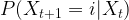
To obtain a time homogeneous Markov chain, we also assume that the matrix K does not depend on the time t. Therefore we define a Markov chain on X to be a sequence $\{X_t\}_t$ of random variables taking values in X with the Markov property saying that for all times t, the conditional distribution for X_t+1 given all previous values $X_0, X_1, \dots, X_t$ only depends on X_t, i.e.

$P(X_{t+1} | X_t, X_{t-1}, \cdots ) = P(X_{t+1} | X_t)$

We also require that this conditional probability is independent of t and is therefore given by a matrix K as in the formula above.

Markov chains on finite state spaces are often visualized as a graph. Suppose, for instance, that our state space contains only two elements: $X = \{ 1 , 2\}$ . We can think of the combined values $X_t$ for all times t as a history of states or as a random walk in the state space. The Markov property then means that the probability to transition into a next state does not depend on the full history, but only on the current state – Markov chains do not have a memory.

In our state space with two elements only, the Markov chain is then described by four transition probabilities: the probability to stay in state 1 when the chain is in state 1, the probability to move to state 2 when being in state 1, the probability to stay in state 2 and the probability to move to state 1 after being in state 2. This can be visualized as follows.

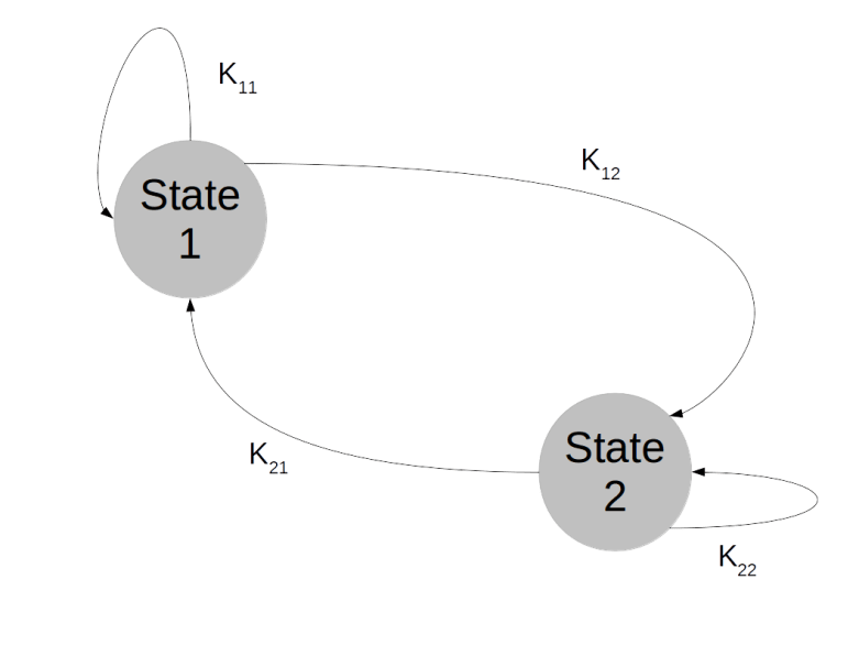
Let us now calculate a few probabilities to get an idea for the relevant quantities in such a model. First, suppose that at time 0, the model is in state j with probability $\mu_j$ . What is the probability to be in state j after one step? Of course we can write

$P(X_1 = i) = \sum_j P(X_1 = i, X_0 = j)$

Now, according to the rules of conditional probabilities, we can express the joint probability as follows.

$P(X_1 = i, X_0 = j) = P(X_1 = i | X_0 = j) P(X_0 = j)$

Plugging this into our previous expression and using the definitions of K and $\pi$ , we now obtain

$P(X_1 = i) = \sum_j K_{ji} \mu_j$

Thus if we think of $\mu$ as a row vector, then the probability after one step is described by the matrix product $\mu K$ .

Now let us calculate a slightly different quantity. Assume that we know that a chain starts at j. What is the probability to be at i after two steps? Using once more the rules of conditional probability and the Markov property, we can write

$P(X_2=i | X_0=j) = \sum_k P(X_2=i | X_1=k)P(X_1=k | X_0=j)$

Intuitively, this is very appealing. To get from j to i in two steps, we can take the way via any intermediate state k. To get the total probability, we simply sum up all these different probabilities! If you have ever seen path integrals in quantum mechanics, this idea will look familiar.

Again, we can write this in matrix notation. Each of the conditional probabilities on the right hand side of the expression above is a matrix element, and we find that

$P(X_2 = i | X_0 = j) = \sum_k K_{ki} K_{jk}$

so that the probability to get in two steps from j to i is simply given by the elements of the matrix K². Similarly, the n-step transition probabilities are the entries of the matrix Kⁿ.

Let us look at an example to understand what is going on here, which is known as a finite random walk on a circle. Our state space consists of N distinct points which we place arbitrarily on a circle. We then define a Markov chain as follows. We start at some arbitrary point x. In each step, we move along the circle to a neighbored point – one point to the left with probability 1/2 and one point to the right with probability 1/2. By the very definition, the transition probabilities do not change over time and depend only on the current state, so is a finite Markov chain. 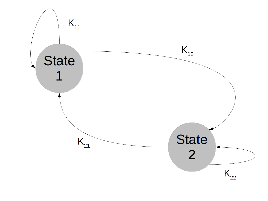If we label the points on the circle by $1, 2, \dots, N$ , then the transition matrix is given by a matrix of the form (for instance for N=4)

$K = \begin{pmatrix} 0 & \frac{1}{2} & 0 & \frac{1}{2} \\ \frac{1}{2} & 0 & \frac{1}{2} & 0 \\ 0 & \frac{1}{2} & 0 & \frac{1}{2} \\ \frac{1}{2} & 0 & \frac{1}{2} & 0 \end{pmatrix}$

More generally, we can also allow the process to stay where it is with probability 1 – p, where p is then the probability to move, which leads us to the matrix

$K = \begin{pmatrix} 1-p & \frac{p}{2} & 0 & \frac{p}{2} \\ \frac{p}{2} & 1-p & \frac{p}{2} & 0 \\ 0 & \frac{p}{2} & 1-p & \frac{p}{2} \\ \frac{p}{2} & 0 & \frac{p}{2} & 1 - p \end{pmatrix}$

Let us try to figure out whether the target distribution, given by the matrix Kⁿ for large n, somehow converges.

To see this, we do two numerical experiments. First, we can easily simulate a random walk. Suppose that we have a function draw which accepts a distribution (given by a vector p whose elements add up to one) and draws a random value according to that distribution, i.e. it returns 1 with probability p₀, 2 with probability p₁ and so on. We can then simulate a random walk on the circle as follows.

def simulate_chain(N, p, steps=100, start=5):
    chain = []
    x = start % N
    chain.append(x)
    for i in range(steps):
        x = (x  + draw([p/2.0, 1.0 - p, p / 2.0]) - 2) % N
        chain.append(x)
    return chain

Here N is the number of points on the circle, steps is the number of simulation steps that we run and start is the starting point. The function draw then returns 1 with probability p/2, 3 with probability p/2 and 2 with probability 1 – p. Thus we move with probability p/2 to the right, with probability p/2 to the left and stay were we are with probability 1 – p. If we set p = 0.8, this results in the following transition matrix.

$\begin{pmatrix} 0.20 & 0.40 & 0.00 & 0.00 & 0.00 & 0.00 & 0.00 & 0.00 & 0.00 & 0.40 \\ 0.40 & 0.20 & 0.40 & 0.00 & 0.00 & 0.00 & 0.00 & 0.00 & 0.00 & 0.00 \\ 0.00 & 0.40 & 0.20 & 0.40 & 0.00 & 0.00 & 0.00 & 0.00 & 0.00 & 0.00 \\ 0.00 & 0.00 & 0.40 & 0.20 & 0.40 & 0.00 & 0.00 & 0.00 & 0.00 & 0.00 \\ 0.00 & 0.00 & 0.00 & 0.40 & 0.20 & 0.40 & 0.00 & 0.00 & 0.00 & 0.00 \\ 0.00 & 0.00 & 0.00 & 0.00 & 0.40 & 0.20 & 0.40 & 0.00 & 0.00 & 0.00 \\ 0.00 & 0.00 & 0.00 & 0.00 & 0.00 & 0.40 & 0.20 & 0.40 & 0.00 & 0.00 \\ 0.00 & 0.00 & 0.00 & 0.00 & 0.00 & 0.00 & 0.40 & 0.20 & 0.40 & 0.00 \\ 0.00 & 0.00 & 0.00 & 0.00 & 0.00 & 0.00 & 0.00 & 0.40 & 0.20 & 0.40 \\ 0.40 & 0.00 & 0.00 & 0.00 & 0.00 & 0.00 & 0.00 & 0.00 & 0.40 & 0.20 \\ \end{pmatrix}$

We can visualize the results if we execute a large number of runs and draw histograms of the resulting positions 100, 200, 300, … steps. The result will look roughly like this (for this image, I have used p = 0.8 and N=10):

We see that after a few hundred steps, this seems to converge – actually this starts to look very much like a uniform distribution. As we already know that the distribution after n steps is given by the matrix Kⁿ, it makes sense to look at high powers of this matrix as well. To visualize this, I will use a method that I have seen in MacKays excellent book and that works as follows.

Visualizing one row of a matrix is not difficult. We can plot the entries in a two-dimensional diagram, where the x-axis corresponds to the column index and the y-axis corresponds to the value. A flat line is then a row in which all entries have the same value.

To display a full matrix, we use colors – we assign one color to each row index and plot the individual rows as just described. If we do this for the powers of the matrix K with the parameters p = 0.8 and N = 10 (and only chose some rows, for instance 1,4,7, to not run out of colors…) we obtain an image like the one below.

We can clearly see that the powers of the matrix K converge towards a matrix

$K^\infty = \lim_{n \rightarrow \infty} K^n$

where all entries in each row seem to have the same value. We have seen that the distribution after n steps assuming an initial distribution described by a row vector $\mu$ is $\mu K^n$ . Therefore the limit distribution is $\mu K^\infty$ . If we take $\mu$ to be a unit vector, we find that the rows of the matrix $K^\infty$ do actually represent the limit distribution of all chains that have started at a specific point i of the state space. Therefore the entries in the rows need to sum up to one, and thus, if they are all equal, need to be equal to 1 / N. If you calculate and print out high powers of the matrix K, you will in fact see that they approach the matrix where all entries are 0.1 (as we have chosen N = 10 in this example).

To completes our short introduction into Markov chains. We have seen that Markov chains model stochastic processes in discrete time in which the state at step t+1 depends only on the state at step t and the dependency is given by a function independent of the current time. In finite state spaces, Markov chains are described by a transition matrix K. The i-th row of the matrix Kⁿ is the distribution of chains starting at point i after n steps. Consequently, converge properties of the Markov chains can be related to converge of high powers Kⁿ and the apparatus of linear algebra can be applied.

In the next post, we will learn more about convergence – how it can be made precise, and how we can tell whether a given Markov chain converges. This will then allow us to construct Markov chains that converge towards a given target distribution and use them for sampling.

Understanding bitcoin blocks

In order to analyse a block, obviously the first thing that we need is – a block. Fortunately, this is not difficult. We can either use the block explorer hosted by blockchain.info to get the second block in the blockchain in raw or JSON or use curl to retrieve the block from the command line, say in raw format.

$ curl https://blockchain.info/de/block/000000006a625f06636b8bb6ac7b960a8d03705d1ace08b1a19da3fdcc99ddbd?format=hex

010000004860eb18bf1b1620e37e9490fc8a427514416f
d75159ab86688e9a8300000000d5fdcc541e25de1c7a5a
ddedf24858b8bb665c9f36ef744ee42c316022c90f9bb0
bc6649ffff001d08d2bd61010100000001000000000000
0000000000000000000000000000000000000000000000
000000ffffffff0704ffff001d010bffffffff0100f205
2a010000004341047211a824f55b505228e4c3d5194c1f
cfaa15a456abdf37f9b9d97a4040afc073dee6c8906498
4f03385237d92167c13e236446b417ab79a0fcae412ae3
316b77ac00000000

For this post, I have chosen a block from the very early days of bitcoin, as this block contains only one transaction and is therefore rather small – current blocks typically contain more than 2.000 transactions and are too long to be displayed easily. This block is actually the third block on the blockchain and has height two. The height is the position of a block on the blockchain (ignoring forks). The block with height 0 is the very first block and actually hardcoded into the bitcoin software, this block is called the genesis block. The first blocks have all been mined (according to their time stamp) in the early morning hours of January 9th 2009.

If you want to follow this post step by step, I recommend to download and run the Jupyter notebook containing the respective code.

In order to understand a bitcoin block, let us again look at the source code of the reference implementation. If you have followed me through the dissection of a bitcoin transaction, you will not have any difficulties to understand the code in primitives/block.h and find that a block is made up of a block header (an instance of CBlockHeader) and the block data which is an instance of the derived class CBlock and contains, in addition to the header fields, the transactions that make up the block. Let us now go through the header fields one by one.

class CBlockHeader
{
public:
    // header
    int32_t nVersion;
    uint256 hashPrevBlock;
    uint256 hashMerkleRoot;
    uint32_t nTime;
    uint32_t nBits;
    uint32_t nNonce;

The first field is the version number, in the usual little endian encoding. Here, the version is simply 1 – not really surprising for the second block that was ever mined. In more recently mined blocks, the version field looks different and is most often 0x20000000 – this is not just a version number any more but a bit mask used to indicate any soft forks that the miner is willing to support, as specified in BIP 009.

The next field is the hash of the previous block. Similar to transactions, this in practice identifies a block uniquely (and is a better identifier than the position in the block chain since it also works for blocks in a fork). Actually, this is not really the hash of the entire block, but of the block header only (GetHash is a method of CBlockHeader).

If we compare the previous blocks hash ID with the JSON output, we find that compared to the JSON output, the order of the bytes is reversed. We have already seen that byte reversal when looking at transactions – the ID of the previous transaction also appears reversed in the serialization compared to the output of a blockchain explorer or the bitcoin-cli tool Time to look at why this happens in a bit more detail.

If you look at primitives/block.h, you will find that the hash of the previous transaction is a uint256. This data type – a 256 bit integer – is defined in uint256.h and is a number. As every number on the x86 platform (on which the bitcoin software was developed), this number is internally stored in little endian byte order, i.e. the least significant bit first (look for instance at the method base_blob::GetUint64 to see this) and is serialized as a little endian byte string (see base_blob::Serialize). However, if it is displayed, it is converted to a big endian representation in the the function base_blob::GetHex(), which simply reverts the order bytewise.

An example where this happens is the JSON RPC server. In blockheaderToJSON in rpc/blockchain.cpp, for instance, we find the line

if (blockindex->pprev)
        result.push_back(Pair("previousblockhash", blockindex->pprev->GetBlockHash().GetHex()));

So we see that GetHex() is called explicitly to convert the little endian internal representation of the hash into the big endian display format. This explains why the order of the hash appears to be reversed in the serialized raw format.

Having clarified this, let us now proceed with our analysis of the raw block data. The next field is called the Merkle root. Essentially, this is a hash value of the transactions which are part of the block, aggregated in a clever way, a so called Merkle tree. We will look at Merkle trees in a separate post, for the time being let us simply accept that this is a hash of the underlying transactions. Again, note that the order of the bytes is reversed between the JSON representation (big endian) and the serialized format (little endian).

The next field is again easy, it is the creation time of the block as announced by the miner who did build the block. As usual in the Unix world, the time is stored as POSIX time, i.e. essentially in seconds since the first of January 1970.

Again, byte order is significant – the hex string b0bc6649 in our case first needs to be reversed and then transformed into an integer:

nTime = nTime = int.from_bytes(bytes.fromhex('b0bc6649'), "little")
import time
print(time.ctime(nTime))

This should give you Friday, January 9th 2009 at 03:55:44.

The next field is called the bits – a name which would probably not win a prize for being a unique, meaningful and descriptive variable name. If you search the source code a bit, you will find that in fact, those bits represent the difficulty which controls the mining process – again, this is a matter for a separate post.

The last field in the header is again relevant for the mining process. It is called the nonce and is used as a placeholder that a miner can set to an arbitrary value in order to produce blocks with different hash values (actually, there is a second nonce hidden in the signature script of the coinbase transaction, we get to this point later when we discuss the mining in detail).

This completes the fields of the block header. In addition to these fields, a full block contains a vector holding the transactions that are contained in the block. As every vector, this vector is serialized by first writing out the number of elements – one in this case – followed by the individual transactions, encoded in the usual serialized format.

With this, we have completed our short tour through the layout of a block and are ready to summarize our findings in the following diagram.

In the next few posts, we will dig deeper into some of these fields and learn how Merkle trees are used to validate integrity and how the difficulty and the nonce play together in the mining process.

Quantum computing and the Blockchain

Browsing the MIT Technology Review, I recently found an article on the potential threat that quantum computing means for the bitcoin protocol in its current form. This article is in fact a review of a paper that appeared last October on the arxiv preprint server. If you use your favorite search engine and search for combinations of words like quantum computing, threat, bitcoin and cryptography, you find many articles on that topic with a greatly varying degree of accuracy – so it is definitely worth taking a look at that paper and see what it really says.

In the bitcoin protocol, computing power enters the picture at two vital points. The first point is the mining process. Recall that in order to create a new block, a mining node has to solve a mathematical challenge called the proof-of-work which is to adjust a part of the new block – the nonce – in such a way that the first few hexadecimal digits of the block hash become zero. The number of digits that need to be zero is controlled by the so called difficulty, a parameter of the network which is dynamically adjusted based on the mining rate, aimining at keeping the mining rate constant at roughly 6 blocks per hour.

So finding the nonce effectively amounts to inverting the used hash function (a double SHA256 hash). Currently, the only (at least publicly) known approach is brute force – simply try out a large number of values for the nonce in parallel and stop when you find a value that solves the puzzle.

On the site blockchain.info, you can find, among much additional information, a graphical history of the difficulty over time. At the time of writing, the development since the birth of the bitcoin looks as follows.

It appears that the difficulty has increased exponentially over the last years (the same web page also offers a version of that graph with a logarithmic scale which demonstrates that starting at 2015, the difficulty did in fact develop essentially exponentially over time). This can be used to estimate the number of hashes per second that are computed by all miners in the network together, and on blockchain.info, there is a nice graph illustrating the result. At the moment, the hash rate is estimated to be roughly 25.000 tera hashes per second, i.e. 2,5 * 10¹⁶ hashes per second, growing exponentially as well.

This dramatic increase in computing power devoted to mining is not just the result of more mining nodes participating in the network. It is also due to an evolution of the technology used to mine bitcoin. In 2010, miners started to use graphical processing units (GPUs), followed by FPGAs about one year later and finally by ASICS, i.e. custom manufactured integrated circuits which can only do one thing – computing hashes – but do this amazingly fast.

In [2], the authors investigate the question at which point in time quantum computing might be developed to the point where a quantum computer can solve the same challenge at a speed that is comparable to currently existing devices. Essentially, their conclusion is that it will easily take between 10 and fifteen years for this to pose a real threat for the bitcoin network. They estimate that quantum computers that can implement the required algorithms will not appear before 2018, and even then the speed of the quantum gates will be much lower than the speed of the custom built ASICS so that it will take in addition at least ten years until a single quantum computers reaches the range of hashing power that the entire bitcoin network represents. Thus, it is unlikely that we will soon see that a single quantum computer is able to run an attack against the bitcoin network based on hashing power.

However, there is a second threat that is much more realistic, targeting the second point in the bitcoin protocol where computing power is essential – the signature algorithm based on elliptic curve cryptography.

In fact, elliptic curve cryptography is based on the difficulty to calculate a discrete logarithm on a classical computer, and was one of the first problems for which it could be shown (see [3]) that it could be solved using a quantum computer much faster, i.e. polynomial in the number of inputs.

In [2], a few attack scenarios are described and one specific scenario is analysed in detail. To understand this scenario, suppose that Alice is creating a transaction to transfer bitcoin to Bob. When she uses the standard P2PKH signature scheme, that transaction will contain the hash value of Bobs public key, but the full public key of Alice. So when this transaction appears on the network, the public key is known. If an attacker is able to solve the discrete logarithm that is required to derive the private key from the public key (see this post for the relation between public and private key), the attacker can use the private key to create an own transaction to spend the UTXO that Alice is using. That attack would have to be executed before the original transaction is added to a block, thus within less than 10 minutes.

The authors then determine how many qubits a quantum computer would need to solve the discrete logarithm and again predict, based on the current rate of improvement of quantum computing technology, how long it would take until a first quantum computer becomes available that can solve this in less than 10 minutes. Different scenarios are considered, but in the most aggressive scenario, this will happen in 2027, i.e. less than ten years from now.

So the conclusion is that the most serious threat to the bitcoin protocol in its current form comes from the anticipated ability of quantum computers to quickly break the ECDSA algorithm in less than ten years from now. Fortunately, the authors also propose countermeasures. In fact, there are public key signature algorithms that appear to be quantum safe, i.e. for which no quantum algorithm is known which can solve the underlying mathematical challenge faster than on traditional hardware. So it is possible to adapt the bitcoin protocol in a way that makes it less vulnerable to attacks by quantum computers.

Thus the key take aways from the paper seem to be that quantum computing will most likely not kill the bitcoin protocol, but force it to change – and that we still have a few years to go even under optimistic assumptions on the rate of further improvement of quantum computing technology.

References

1. L. Cocco, M. Marchesi, Modeling and Simulation of the Economics of Mining in the Bitcoin Market, PLoS One 11 (10) (2016)
2. D. Aggarwal et al., Quantum attacks on Bitcoin, and how to protect against them
3. P. W. Shor. Polynomial-Time Algorithms for Prime Factorization and Discrete Logarithms on a Quantum Computer. SIAM Review, 41(2):303–332, 1999 (see also the preprint on the arxiv)

Monte Carlo methods and Markov chains – an introduction

In our short series on machine learning, we have already applied sampling methods several times. We have used and implemented Gibbs sampling, and so far we have simply accepted that the approach works. Time to look at this in a bit more detail in order to understand why it works and what the limitations of the algorithm are.

Regardless of whether you want to simulate ferromagnetic behavior in an Ising model, run a Hopfield network or train a Boltzmann machine, the fundamental problem that we have to solve is always the same. We are given a probability distribution P living on some state space X, and we are trying to create a sample, i.e. a set of points in the state space such that the probability for a point x to appear in this sample is equal to the probability P(x) given by the probability distribution.

The naive approach to this is simple: visit every point x in the state space and include that point with probability P(x). However, it is clear that with a large state space, this approach is not computationally feasible. In the example of a Boltzmann machine trained on handwritten digits with 28 x 28 pixels, our state space has 2⁷⁸⁴ elements, and there is no way we can visit them all one by one. Instead, we would need something like a randomized walk through the state space. We could start with same randomly chosen state X₀, then – using a randomized transition rule – move on to a point X₁ and so forth. Intuitively, we want to select our transition rule in such a way that the state space elements X_i selected in this way form a sample, i.e. such that our chain of state space locations visits regions with large values for P(x) more often than regions with low values of P(x). Thus we would systematically ignore regions of the state space with low probability which would greatly reduce the number of states that we have to visit to obtain a valid sample.

So, from a mathematical point of view, we consider a sequence of random variables X_i such that X_i+1 is related to X_i by some randomized transition rule. We also assume that this rule does not depend on the index i which is usually called the time. Thus we have a sequence of random variables X_i which is not independent, but almost independent – X_i+1 depends only on X_i and in way that itself does not vary with i. This is called a Markov chain (more precisely, a time homogeneous Markov chain).

Let us consider an example to illustrate the idea. As our state space, we choose the space or real numbers. We fix a starting value, say X₀=0, and we obtain the next value by adding a number that we draw from a standard normal distribution. Thus, mathematically, we assume that W_n are identically distributed and independent random variables, all distributed according to the standard normal distribution, and set

$X_{n+1} = X_n + W_n$

This is a Markov chain: the value X_n+1 depends only on X_n, not on any earlier elements of the chain. The transition rule is randomized, but itself does not depend on the time step n – all W_n have the same distribution. Let us implement this in Python to see how it works (the full notebook can be downloaded here).

Sorry, something went wrong. Reload?

Sorry, we cannot display this file.

Sorry, this file is invalid so it cannot be displayed.

view raw GaussianRandomWalk1.ipynb hosted with ❤ by GitHub

Here we have created and displayed three different random walks. All of them start at the same point (zero), and all of them follow the same transformation rule, but as the transformation rule is stochastic in nature, they all develop differently.

Now let us try to turn the view on this upside down. This time, we execute a larger number – 1000 – of random walks with 5000 steps each. But instead of plotting the sequence of points X_i for every walk, we display the distribution of the last point of each walk, i.e. we plot the distribution of the random variable X₄₉₉₉.

Sorry, something went wrong. Reload?

Sorry, we cannot display this file.

Sorry, this file is invalid so it cannot be displayed.

view raw GaussianRandomWalk2.ipynb hosted with ❤ by GitHub

This does in fact look more familiar. We see that most walks end up being close to zero at the end – steps in the positive direction and steps in the negative direction cancel each other. Only very few walks end up at an extreme position close to plus or minus 200 – this is not surprising as well, to arrive at an extreme point, we would need to draw 5000 times in a row an extreme value from the random normal distribution, which is a rather unlikely chain of events.

In this case, the distribution does actually not converge if we increase the number of steps – you can try this out and play with different values, i.e. replace 5000 by 50000 (this will run some time) and look at the distribution of X₄₉₉₉₉ – you will see that this is now spread out to roughly plus / minus 750 (in fact, the distribution is obtained as a multiple convolution of the standard normal distribution with itself and thus is again a normal distribution).

Even though the distribution does not converge, we have been able to sample from a specific distribution – in this case the distribution after 5000 steps – using only the ability to sample from a different distribution – in this case the random normal distribution. Obviously, in this special case, the result is trivial, but the principle that we have found looks interesting. Can we generalize this approach to obtain sampling methods for target distributions that are otherwise intractable?

Now this is exactly the idea behind the sampling approach that is commonly known as Markov chain Monte Carlo (MCMC) and which has become very popular, with applications to complex simulations in theoretical physics, to machine learning and even asset pricing and value-at-risk calculations.

So let us summarize how the MCMC approach works. Given a target distribution P(x), we first construct a Markov chain that converges to that target distribution. Once we have that, we can simulate a large number of runs and use the resulting points as our sample (in fact, in many cases we can also do with one run only, as we will see later). Thus in order to utilize Markov chains for sampling, we would need to understand under what conditions a Markov chain converges and if it converges, how we can relate the target distribution to the transformation rule. We will look into these points in more detail in future posts in this series.

Bitcoin mining – an overview

In my recent posts in this series, I have walked you in detail through two of the basic objects that make up the bitcoin blockchain – participants, represented by public / private key pairs, and transactions. Time to look at the third major ingredient – blocks.

What are blocks and why are they necessary? When the bitcoin protocol was invented in 2008 by a person (or group of persons) acting under the pseudonym Satoshi Nakamoto (see [1]), the real novelty was not the usage of a chain of transactions in order to model payments. The real novelty was the proposed solution for a major issue with a cryptocurrency that is based solely on such a chain: the problem of double spending. To understand this, suppose that Eve agrees on a deal with Alice: Eve will transfer a certain amount of bitcoin to Alice in exchange for another currency like USD. She would pick an unspent transaction output of the correct amount, create and sign a transaction and publish that transaction in the network. Alice could see and validate the transaction appearing in the network and would then transfer the USD amount to Eve.

Unfortunately, Eve could, at virtually the same time, agree on a similar deal with Bob and create another transaction transferring the same unspent output to Bob.

Now we have two transactions in the network that both claim to spend the same previously unspent transaction output. However, what if, due to some network latency, Bob and Alice detect the second transaction only after they have initiated the transfer of the USD amount? And if they detect the problem, how can they – and the entire network – agree on which of these transactions should be considered valid and which should be discarded? This is the double spend problem.

To solve this, a mechanism is needed that allows all nodes of the network to agree on an order of transactions. If we have that order, the solution to our problem is easy – the first transaction, i.e. the transaction with the lowest order wins. Satoshis proposal was to implement an ordering by what he called a timestamp service and what is now known as the blocks of the blockchain.

Essentially, blocks are groups of transactions. Nodes in a bitcoin network collect transactions that have been posted, but not yet included in a block. They then calculate hash values of these transactions and organize them into a larger data structure – the block. But similar to transactions, blocks are linked into a chain – Satoshi calls this proof-of-work chain and in fact the term blockchain does not appear at all in his paper but was introduced later. Each (full) node in the network maintains a local copy of this chain. Whenever a node creates a block, it includes the hash value of the current last block in the chain in the block data structure. It then publishes the block on the network. If other nodes pick up the block, they can verify that it is valid – in particular they can verify that none of the transactions included in the block lead to double spending with respect to any other transaction in this or earlier blocks. If this validation is successful, the block is added to the copy of the chain maintained by the server.

The fact that the blocks in the chain are linked makes it more difficult to alter a block (and the transactions contained in it) that is already buried below some new blocks. In fact, in order to do this, we would have to recreate all blocks between the current last block and the block that we want to alter, as the blocks contain hash values of their predecessor. In order to make sure that this is virtually undoable, every node that creates a block needs to solve a mathematical puzzle – a so called proof of work. The difficulty of this puzzle can be adjusted dynamically and is kept at a level where approximately 10 minutes of work are required to create a new block. This also makes it less likely that new blocks are created at exactly the same point in time.

In the bitcoin block chain, this proof of work is designed as follows. The block data structure contains hash values of the transactions that are part of the block and – in addition – a field called the nonce that the node creating the block can determine at will. As the nonce enters the hash value of the block, this implies that, simply by trying out different values for the nonce, a node can create blocks whose hash value has certain properties. The mathematical challenge that a node has to solve to create a block that is accepted by the network is to adjust the nonce such that the hash value of the block is zero in the first few hexadecimal digits. The number of leading digits that need to be zero is the difficulty which is adjusted over time to make sure that the block creation rate is kept at one block per ten minutes.

Thus a node that wishes to create a new block will collect transactions not yet included in a block, verify them (and will thereby avoid double spend), add them to a block along with the hash of the current last block, try out some value of the nonce, calculate the hash value, check whether its first digits are zero, try a different nonce if that is not the case and so on until a matching nonce is found. Then the block is published, verified by the other nodes and – if it passes the checks – added to the block chain as the next block. Nodes that create new blocks are called miners.

Let us now trace the full history of a sample transaction throughout this process.

Suppose Alice wants to transfer 50 BTC to Bob. She creates and signs a transaction according to the rules that we have seen in the previous posts. That transaction is then published in the network. A mining node picks up the transaction and assembles it – along with many other transactions – in a new block. That block is then distributed on the network. Each node on the network validates the block and adds it to the copy of the blockchain that this node maintains. Finally, Bob can listen on the network as well. As soon as Bob finds that the transaction has been added to a block and this block has been included in the network, he can be relatively sure that the transaction is valid. Bob can now be confident to be protected against double spend and use this transaction in turn as unspent output (as a rule of thumb, a transaction is considered to be confirmed if it is included in a block and at least five additional blocks have been added on top of that, i.e. after roughly one hour).

There are still a few open ends. Why, for instance, should a mining node invest CPU power in the creation of blocks? And what happens if two different blocks are mined at the same time?

Let us first start with the question of incentivation. In order to make sure that miners participate in the process, a miner is rewarded for every block that he creates. In fact, each new block contains a special transaction called a coinbase transaction. Such a transaction has no inputs, and the mining node can determine the address to which the output is credited. Thus, effectively, mining creates bitcoins, and the miner earns the newly created bitcoins.

The amount of a coinbase transaction used to be 50 BTC in the first days of the bitcoin protocol, and is halved every 210.000 blocks. At the moment, the reward is 12.5 BTC, which is the equivalent of roughly 10.000 USD at the current exchange rate. This is the incentive for the mining node to invest energy and hardware cost into the process.

Now let us see what happens if two valid blocks are mined at the same time. In this case, we create a fork of the chain.

Suppose, for instance, that two different nodes find a solution for the mathematical puzzle at exactly the same point in time and publish two blocks that could fit into position N of the chain. Let us call these blocks N and N’. Now all the other nodes in the network have to take a decision which chain they consider to be the main chain – the chain continued with N or the chain continued with N’. There is one basic rule in this game – the longest chain wins. However, at this point in time, both chains have the same length. So some of the nodes – say roughly half of them – will opt for the first chain, the other part of the nodes will opt for the second chain. Now each mining node will continue to work on the chain that this node considers to be valid. So roughly 50% of the miners will start to work on a block which could follow block N and the other nodes will start to search for a block that could follow N’.

Now it is rather unlikely that again, both puzzles are solved at exactly the same point in time. So let us assume that the next block which is mined is based on N. This block will then be published. Now the chain based on N is longer than the chain based on N’, and all the other nodes will – according the rule that the longest chain is the winning chain – discard the chain based on N’ and continue to mine blocks based on the new chain that included N. Thus the fork is resolved and all chains agree again on one copy of the chain.

That completes our short overview of the mining process. In the next couple of posts, we will again analyze the structure of a block in detail and see whether we will eventually be able to mine and publish a block in our test network.

References

1. Satoshi Nakamoto, Bitcoin: A Peer-to-Peer Electronic Cash System, 2008
2. Bitcoin History: Pre-Blockchain Digital Currencies