Factoring integers on a quantum computer with Qiskit

After all the work done in the previous posts, we are now ready to actually implement Shor’s factoring algorithm on a real quantum computer, using once more IBMs Q Experience and the Qiskit framework.

First, recall that Shor’s algorithm is designed to factor an integer M, with the restriction that M is supposed to be odd and not a prime power. Thus the smallest meaningful value of M is M=15. Of course this is a toy example, but we will see that even this toy example can be challenging on the available hardware. Actually, 15 is also the number that was factored in the first implementation of Shor’s algorithm on a real quantum computer which used an NMR based device and was done in 2001 – see [1].

The quantum part of the algorithm is designed to find the period r of a chosen number a modulo M. There are several choices of a that are possible, the only condition we need is that a and M are co-prime. In this post, we follow the choice in [1] and use a = 11 and a = 7. As in [1] (and all other similar papers I am aware of, see also the discussion in this paper by Smolin, Smith which later appeared in Nature) we will also rely on prior knowledge of the result to build up our circuits, so we are actually cheating – this is not really an application of Shor’s algorithm, but merely a confirmation of a known factoring.

Of course, it is easy to compute the period directly in our case. The period of a = 11 is two, and the period of a = 7 is four. A smaller period means a simpler circuit, and therefore we start with the case a = 11. Let us see whether we can confirm the period.

The easy case – a = 11

For our tests, we will use the description of Shor’s algorithm in terms of the quantum phase estimation procedure. Thus we have a primary register that we initialize in the state and to which we apply a sequence of controlled multiplications by powers of a, and a working register, in which we do a quantum Fourier transform in the second step. The primary register needs to hold M=15, so we need four qubits there. For the working register, we use three qubits, which is the smallest possible choice, to keep the number of gates small.

The first step of our algorithm is controlled multiplication by a. However, this is greatly simplified by the fact that we apply this to exactly one state that we know upfront – the initial state . Thus we only need to implement a unitary transformation which conditionally maps the state to the state . In binary notation, eleven is 1011, and we therefore simply need to conditionally flip qubits 3 and 1. We also need a Pauli X gate in the primary register to build the initial state from the fiducial state and Hadamard gates in the working register to create the initial superposition. Thus the first part of our circuit looks as follows.

What about higher powers of a? This is easy – we know that a² is equal to one modulo M, and therefore the multiplication by a² modulo M is simply the identity transformation. The same is true for all even powers and so we are already done with the first part of our circuit – this is why we call the case a = 11 the easy case. The only thing that is left is to add the quantum Fourier transformation and a measurement to the working register. This gives us the following circuit (which can obviously be simplified, more on this later).

Now we can run this on a simulator. Before we do this, let us try to understand what we expect. We know that after measuring the working register, the value that we obtain is a multiple of 2³ / r = 8 / 2 = 4. Thus we expect to see peaks at 0 and four (binary 100). And this is actually what we get – the following histogram shows the output of an execution on the local QASM simulator integrated into Qiskit.

This is nice, our circuit seems to work correctly. So let us proceed and try this on real hardware. Before we do so, however, let us simplify our circuit a bit to reduce the number of gates needed and thus the noise level. First, we skip the final swap gates in the QFT circuit – this will change our expected output from 100 to 001, but we can keep track of this manually when setting up the measurement. Next, we have two Hadamard gates on w[2] that cancel and that we can therefore remove. And the Pauli X gate on p[0] is never really used and can be dropped. After these changes, we obtain the following circuit.

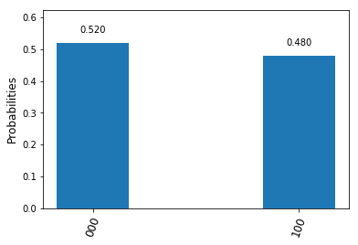
We can run this on the IBMQ hardware. As we require seven qubits in total, we need to do this on the 14 qubit model ibmq_16_melbourne. Here are the results of a test run, again as a histogram.

We see the expected peaks at 000 and 100, but also see some significant noise that is of course not present in the simulation. However, the probabilities to measure one of the theoretically expected values is still roughly twice as high as the probability of any of the other values.

The hard case – a = 7

Having mastered the case a = 11, let us now turn to the case a = 7. The only change that we need to make is the circuit acting on the primary register. In the first part of the circuit, we can again make use of the fact that we only have to deal with one possible input, namely the initial state . The conditional multiplication by a maps this to , and we can again implement this by two conditional bit flips, i.e. two CNOT gates.

The second part, the conditional multiplication by a² = 4 modulo M, requires a bit more gates. On a bit level, multiplication by four is a bit shift by two bits to the left. We can realize this as a sequence of two conditional swap gates, swapping the bits zero and two and the bits one and three. A conditional swap gate can be implemented by three CNOT gates, or, in QASM syntax,

gate cswap a,b,c
{
  cx c,b;
  ccx a,b,c;
  cx c,b;
}

We can also make a few simplifications by replacing CNOT gates with fixed values of the control qubit by either an inversion or the identity. We arrive at the following circuit.

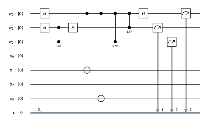
This is already considerably more complex than for the case a = 11. When we add the QFT circuit and the measurements, we end up with the following circuit.

Now the period is four. Thus we expect peaks at all multiples of two, i.e. at all even values. And this is actually what we get when we run this on a simulator.

Now let us again see how we can optimize this circuit before trying it on real hardware. Again, there are a few additional simplifications that we can make to reduce the noise level. On w[2], we have a double Hadamard gate that we can remove. We can again dispose of the final swap gates and move the swap operation into the measurement. The last CNOT between p[1] and p[3] can be dropped as it does not affect the outcome. The same is true for the last CNOT between p[0] and p[2]. Thus we finally arrive at the following circuit.

And here is the result of running this on the 16 qubit IBM device.

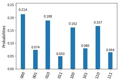
Surprisingly, the noise level is not significantly worse than for the version with a = 11, even though we have a few more gates. We can clearly see that the probabilities to measure even values are significantly higher than the probabilities to measure odd values, corresponding to the period four.

So what did we learn from all this? First, our example was of course a toy model – we did code the circuit based on knowledge on the period and hard-coded the value of a. However, our example demonstrates the basic techniques to build circuits for the more general case. In real application, we could, given a number M, first determine a suitable value for a. The conditional multiplication by a is then acting as a permutation on the computational basis and can therefore be implemented by a sequence of (conditional) swap gates. The same is true for higher powers of a. So in theory, we have all the ingredients that we need to implement more general versions of the algorithm.

In practice, however, we will quickly reach a point where the number of gates exceeds the limit that we can reasonable implement given the current level of noise. So real applications of the algorithm in number ranges that are not tractable for classical digital computers will require advanced error correction mechanisms and significantly reduced noise levels. Still, it is nice (and fun) to see a toy version of the famous algorithm in action on a real device.

If you want to run the examples yourself, you can use my notebooks for the case a=11 and a=7.

References

1. L. Vandersypen, M. Steffen, G. Breyta, C. Yannoni, M. Sherwood, I. Chuang, Experimental realization of Shor’s quantum factoring algorithm using nuclear magnetic resonance, Nature Vol. 414, (December 2001)
2. P. Shor, Polynomial-Time Algorithms for Prime Factorization and Discrete Logarithms on a Quantum Computer, SIAM J.Sci.Statist.Comput. Vol. 26 Issue 5 (1997), pp 1484–1509, available as arXiv:quant-ph/9508027v2
3. R. Cleve, A. Ekert, C. Macchiavello, M. Mosca, Quantum Algorithms revisited, arXiv:9708016
4. A. Kitaev, Quantum measurements and the Abelian Stabilizer Problem, arXiv:quant-ph/9511026
5. J. Smolin, G. Smith, A. Vargo, Pretending to factor large numbers on a quantum computer, arXiv:1301.7007 [quant-ph]