ctOS – LeftAsExercise

Accessing your hard drive – the OS developers moment of truth

When building your own operating system, the moment when you first write data to a real physical hard disk of a real PC is nothing less than thrilling – after all, making a mistake at this point could mean that you happily overwrite data on your hard drive randomly and wipe out important data on your test machine.

So working with real hard drives is nothing for the faint of heart – but course, no operating system would be complete without that ability. In this post, we look at the basic concepts behind the communication between the operating system and the hard drive.

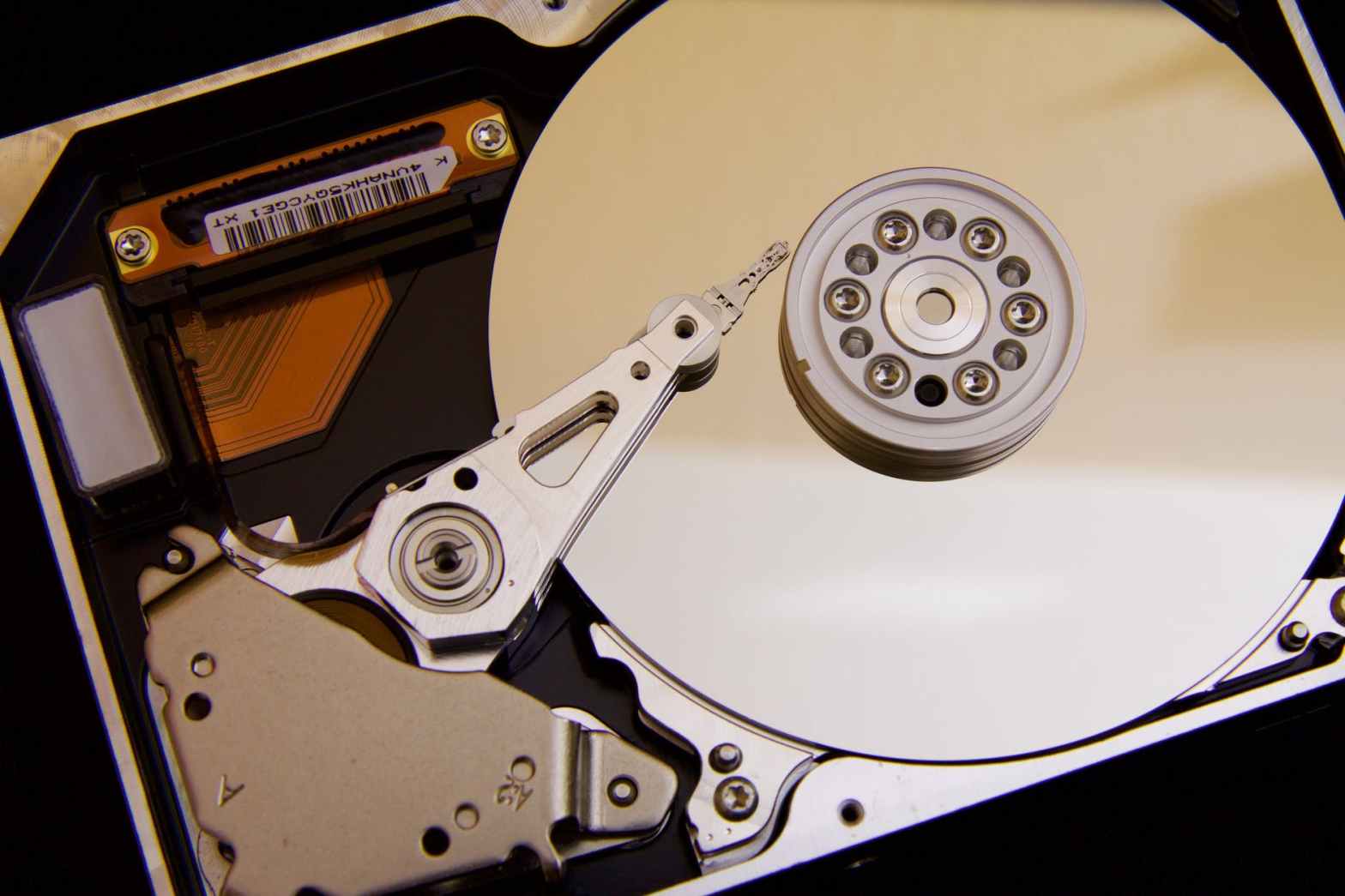
First, let us see how data on a hard drive is stored. The most basic conceivable hard drive consists of a thin disk, called a platter, on which the data is stored, and a device called head that is able to read and write data. The disk is spinning and the head can be moved forth and back across the disk, so that it can be positioned at an arbitrary distance from the center of the disk.

Physically, the disk is organized in concentric tracks. When the head is positioned at a certain distance from the center of the disk, it can therefore access an individual track. Tracks are further separated into sectors, as shown in the upper part of the diagram below (taken from this Wikipedia page). Finally, a block is the intersection of a sector with a track. So to identify a specific block, you could use the combination of a sector and the track on which the block is located.

This simple design is actually wasting some space, as you could only use one side of the disk. If you want to store data on both sides, you need two heads – one below and one above the disk. You could even increase the capacity further by building a stack of platters, which heads being located between the platters so that each side of a platter corresponds to one head reading from it and writing to it, as displayed in the lower part of the diagram.

In this setup, the union of tracks locates at corresponding positions on all platters is called a cylinder. If you know the cylinder and the head, you know the track. You could therefore specify the location of a block on the disk by the combination of a cylinder, a head and a sector. This addressing method is therefore called the CHS addressing and was the first addressing mode used on early IBM PCs and compatible machines.

Later, the actual geometry of the hard drive became more complicated, and addressing schemes that decouple the actual geometry of the hard drive from the address were introduced, most notably the so-called logical block addressing (LBA). In that addressing mode, which is the current standard, a hard disk is thought of as a sequence of blocks, numbered starting with zero. To access a block, you simply specify the number of the block. The hard disk controller, i.e the circuitry that is actually operating the hard drive and sitting between the CPU and the actual hard drive, will convert this LBA number into the actual physical location of the data on the drive.

So how do we actually access a block? The easiest way to do this is usually called programmed input output (PIO). To explain this, we first need to recall that a CPU is not only accessing the system memory, but can also talk to devices using designated channels, so called ports. If the CPU writes to a port, the data will be sent to the device, and vice versa data written by the device can be accessed by the CPU by reading from a port.

So to read from a hard drive, we could proceed as follows. First, we would write a command to a specific port associated with the hard drive. This command would tell the hard drive what to do – for instance to read – and it would contain the LBA number of the block we want to read. Then the hard drive controller would perform the actual read operation, and once complete, would send the data back to the CPU that would then read it from a port.

The format of the commands and the exact interaction between the CPU and the device in this process were defined in a standard called ATA, also called IDE or Parallel ATA (PATA). This specification did not only describe the interaction between the hard disk controller and the CPU, but also the low-level electronics, cables, connectors and so forth.

This method of reading and writing data is simple, but has a major disadvantage – it keeps the CPU busy. In the worst case, the CPU has to write the command, wait in a busy loop and then read the data one word at a time – and if you wanted to read several blocks, you had to do this over and over again. Not surprising that alternatives were developed soon.

The first improvement we can make is to make the operation interrupt driven. In this version, the CPU would send a command and could then go off and do something else while the hard disk controller is working. Once the data has been read, the controller informs the CPU that data is available by raising an interrupt, and the CPU can go ahead and fetch the data. This is already more efficient, but still suffers from the fact that the data has to be read byte for byte.

Consequently, the next step in the development was what is called Direct Memory Access (DMA). With DMA, the hard disk controller can communicate directly with the memory controller and transfer the data read directly into a designated area of the systems main memory without any involvement of the CPU. Only once all the data has been read, an interrupt is raised to raised to inform the CPU that the data has been transferred and can be worked with. With this approach, large blocks of data can be read and written while the CPU is able to work on other threads.

In 2000, a serial version of the ATA standard called Serial ATA (SATA) was introduced. Due to the serial processing, SATA allows much higher transfer rates between the hard drive and the motherboard and therefore a much higher I/O throughput and soon involved into the de-facto standard, also for consumer PCs. A SATA device can still operate in a so-called legacy mode, where it is presented to the CPU as a PATA/IDE device. However, to take advantages of some new features of the SATA protocol, for instance a higher number of devices per controller, a new protocol for the communication between the CPU and the controller needs to be used which is called AHCI. The AHCI protocol is significantly more complicated than the ATA protocol, but in fact both protocols still follow the same logical steps to read and write data.

Let us now combine this understanding with what we have learned about interrupts and multitasking to see how the operating system would typically orchestrate a disk drive access, for instance to read data from the disk. The following diagram illustrates the process.

First, the operating system reserves an area of system memory for the DMA transfer. Then, the kernel prepares the command. The format of the command depends on the used protocol (AHCI or legacy IDE), but typically, the command would encompass the location of the data on the disk to be read, the number of blocks to be read and the location of the DMA buffer. Then the command is sent to the hard drive.

At this point in time, the CPU is free to work on something else, so the kernel would typically put the current task to sleep and re-schedule so that a different task can start executing.

While this happens, the hard drive starts to execute the command. It reads the requested data and places it in the DMA buffer prepared by the OS. Then it raises an interrupt to indicate that the data has arrived in main memory.

Once the operating system receives the interrupt, it will stop the currently executing task and switch back to the task that requested the read. This task can now continue execution and work with the data.

Of course, the real picture is more complicated. What the image above calls the “device”, for instance, is in reality a combination of the actual hard disk controller and components of your motherboards chip set, like the AHCI controller or the DMA controller. In addition, several hard drives can operate in parallel, so the kernel needs a way to keep track of the currently executing requests and map incoming interrupts to the requests currently in flight. And, in an SMP environment with more than one CPU, semaphores or other locking mechanism need to be in place to make sure that different requests do not collide. If you are interested in all those details, you might want to take a look at the documentation of the ctOS hard disk driver.

We now understand how a hard drive and an operating system kernel communicate to read or write sectors. However, an application does of course not see individual blocks of a hard disk, instead the hard disk appears as a collection of files and directories. The translation between this logical view and the low-level view is done by the file system at which we will look in the next post in this series.

How does multitasking really work?

The first PC on which I was running a copy of Linux back in the nineties did of course only have one CPU, so it was clear to me that it could physically only execute one instruction at a time – but still, it magically created the impression to run several programs in parallel without visible delay. How could that ever work? Almost twenty years later, I finally found the answer.

In fact, trying to understand how multitasking and multithreading actually work was one of my main motivations when I developed the ctOS kernel a couple of years ago. In this post, I will try to explain the basic mechanism behind the magic.

The basic idea sounds simple enough. Suppose a task has been running for some time and the operating system decides that it is time to switch to a different task. Then the operating system kernel will interrupt the current execution and save the current state of the CPU somewhere in memory. It then locates a different task that is ready to be run – a process which is called scheduling– and retrieves the saved CPU state representing this task from memory. Then, it will let the CPU continue execution with that saved state. As this state is exactly the state of the CPU that was in place when the newly scheduled task was stopped, the CPU will continue to process this task as if it had never been interrupted.

Unfortunately, this simple explanation leaves a number of questions open. First, if a task is executing, it means that the CPU is busy running this task. How, then, can the operating system “do” something? Second, what is the “state of the CPU”? How can we store it and how can we put the CPU back in a saved state? And then, how do we decide that “it is time to switch to a different task”? It turns out that the answer to these questions have to do with interrupts.

Task switching, interrupts and the stack

To explain this, let us for a moment assume a vastly simplified world where all tasks currently active do not require I/O operations. Suppose task A is currently being processed, i.e. the CPU is executing the stream of instructions (the “program”) that make up this task. At some point, we will see an interrupt firing. If there is no I/O, this is usually the timer interrupt that fires periodically, say one thousand times per second.

If this happens, the CPU will stop the execution of task A and start to execute an interrupt service handler. Now the interrupt service handler has been set up by the operating system and points at code within the operating system kernel – so at this point, control is given to the operating system! At the same time, we have learned that the CPU will store the value of some registers like EIP on the stack, and a smart interrupt handler will store the value of additional registers on the stack as well in order to be able to use and reconstruct their value later, and, right at its end, contain code to pop the register values off the stack again. So we could as well set up our ISR in such a way that it does in fact store the value of all registers on the stack. This already provides two ingredients for the task switching mechanism – a way to make sure that the operating system gains control of the CPU at least once a millisecond and a saved CPU state on the stack!

Now the operating system will usually maintain a list of tasks and scan that list according to certain criteria to find a task which should be executed next – we will look at this process in greater detail further below. Suppose that it determines a task which we call B which should be run next. For the sake of simplicity, let us also assume that this task is not entirely new, but has already been running for some time (setting up a new task is a bit more complicated). Thus, when task B was interrupted for the last time, its state was also saved on the stack somewhere, and our operating system has hopefully stored a pointer to this stack.

What we now want to do is to exchange the stored state of task A with that of B. The easiest way to do this is not to copy around the stacks, but to manipulate the stack pointer such that the execution resumes using the stack of task B instead of task A! When we do this and reach the end of the interrupt service handler, the part of the interrupt service handler that is responsible for popping all registers off the stack again as well as the final IRET will use the stack of task B. In other words, the CPU will pick up the state of task B instead the state of task A. It will therefore continue execution with the state of the registers and the instruction pointer that task B had when it was interrupted – in other words, task B will continue to execute instead of task A, and we have switched from task A to task B.

In reality, there are a few subtle points that need to be worked out in more detail when you really want to build this. You will have to think about what the stack actually is – does every task have its own stack, how do you isolate them etc. In addition, a task switch might invoke a switch to a different process and thus to a different virtual address space, so at some point, addresses become invalid and cannot be accessed any more. The exact process that ctOS uses is described in the section on task switching in the interrupt handling documentation of ctOS.

We have explained the process of task switching using the timer interrupt as an example. However, this is not the only possible trigger for a task switch. There are of course other hardware interrupts that might trigger a task switch, but more importantly, many task switches do in fact occur during a system call! Assume for instance that a task wants to read data from the hard drive. It will then invoke a system call to do this, i.e. it will hand over control to the kernel voluntarily. The kernel will ask the hard drive to go and get the data, but of course this takes some time. Thus the kernel will in general not return to this task, but schedule a different task and execute a task switch. If (as ctOS does it) a system call is itself implemented as a software interrupt, the mechanism is exactly the same as if a task switch had been done during the processing of a hardware interrupt (if the faster SYSENTER/SYSEXIT mechanism is used, the processing is a bit different but the idea is the same).

Scheduling

What we have not explained so far is how the operating system does actually select a new task to be executed. The exact details how to do this are different for each operating system, but it is probably fair to say that there are in general two main ingredients – the time the task has been running until the last task switch and the state of the task.

First, there is the CPU time that a task has consumed since the last task switch, commonly measured by the quantum. The quantum is a number that is set to some initial value when the task gets control of the CPU. During each processing of the timer interrupt, the quantum of the currently active task is decreased by one. As the timer interrupt fires periodically, the quantum thus measures the time that the task has already consumed – the lower the remaining quantum, the longer the task did already run. If a task has reached quantum zero, it might be a good idea to schedule a different task.

Second, there is the state of a task. Not every task is ready to be executed at any given point in time. A task might for instance be waiting for some event (user input, I/O, ..) or might otherwise be blocked. Our a task could be in the status new, indicating that it is currently still being set up and not yet ready to run. Or it might have been stopped by a signal and be waiting for the signal to continue. And finally, a task can either be active i.e. currently executing, or ready, i.e. waiting to be scheduled.

During scheduling, only tasks in status ready will be considered as candidates for execution. One way to implement scheduling is to put all ready tasks onto a queue, called the ready queue. Scheduling than basically proceeds as follows.

Check whether the currently active task has used up its quantum
If no, decrease the quantum by one and return – no task switch will be done. Otherwise proceed with the next step
Set the state of the currently active task to “ready”, set its quantum back to its initial value and queue the task at the end
Select the first task in the ready queue. Update its status to active and mark it as target of the next task switch

When a task that was not ready but, for instance, blocked, becomes ready, it is added at the end of the ready queue with an initial quantum.

There is a more advanced version of this simple algorithm called round-robin scheduling with dynamic priorities. In this model, there is more than one ready queue, in fact there is a list of priorities, say 0 – 15, and there is one queue for each priority. If a new task to be scheduled needs to be determined, these queues are scanned for candidates, starting with the highest priority queue. The priority can be adjusted at run-time based on the current behaviour of the process – see the documentation of the ctOS scheduler for more details. This approach is still comparatively simple, and designing a highly optimized scheduler is an art that can make the difference between a good and a lousy performance. Currently, Linux uses a different scheduling mechanism called CFS, but scheduling remains a tricky tasks, especially in an SMP environment, and we will probably see additional work going into this in the future (see for instance this article for a more in-depth discussion).

Now multi-tasking is nice, but to really execute several programs at the same time has an additional dimension – memory. If you want to run different programs on one physical machine that might even belong to different users, you need to make sure that a program cannot access memory reserved for a different program, i.e. you need some level of memory space isolation. Fortunately, modern CPUs offer a mechanism called virtual memory that we can use for this purpose and that we will explain in the next post.

Interrupts – the heartbeat of a Unix kernel

Modern operating systems are mostly event driven – network cards receive packets, users hit keys or a mouse buttons, built-in timer create events or data arrives from a hard drive. To be able to process these events, a CPU needs a mechanism to stop whatever it is currently doing and run some code designed to deal with the event – and this is what is called an interrupt.

How do interrupts work?

Formally speaking, we could define an interrupt as an event that instructs the CPU to stop the current flow of processing, jump to a defined location in memory, execute the instructions there and later, when that stream of instructions is complete, resume processing at the point where it left of.

To understand how this works, let us briefly recall some basic concepts in CPU design. First, remember that a CPU has – apart from other units – a certain set of registers, i.e. a set of easily accessible, but small pieces of memory that the CPU uses to store intermediate results of a calculation. To be a bit more specific, let us assume that we talk about an x86 CPU in protected mode. Then there are registers called EAX, EBC, ECD and EDX (and many others) that can hold 4 bytes, i.e. 32 bits, each. Instructions like the ADD command can refer to these register and, for instance, add the content of two registers and store the result in a third register.

In addition to these general purpose registers, there are a few other special registers. One of them is the register called EIP which is the instruction pointer – it points to the memory location where the instruction just executed is stored. And there is the stack pointer ESP, which points to the bottom of the stack, i.e. to an area of memory which a program can use to temporarily store data. When a program pushes data on the stack, the stack pointer is decremented, i.e. the stack grows downwards, and the data it is written to the memory location to which the stack pointer then refers. If a program pops data from the stack, the data is taken from the memory location to which the stack pointer currently refers, and the stack pointer is incremented again.

When instructions are executed one by one, the instruction pointer is simply increased after the processing of one instruction has been completed to point to the next instruction. However, when a program uses the CALL instruction to call a subroutine, the CPU will have to continue execution not at the next instruction, but at the start of the subroutine. When the subroutine completes, however, it needs to resume processing at the next instruction after the CALL instruction. So it has to save this address – called the return address – somewhere.

As there is only a small set of registers available and we might want to do nested calls, the CPU cannot use a register for this purpose, so it uses the stack. Thus, if we call a subroutine, the return address is pushed onto the stack. When the subroutine has completed, a special instruction called RET is placed in the code. This instruction tells the CPU to get the return address from the stack and resume execution at this point.

By now, you might be asking yourself why I am telling you all this. The answer is simple – interrupts work in a very similar way. In fact, when an interrupt is raised (we will see further below what this actually means), the CPU places the current value of the EIP register on the stack. It then jumps to a predefined point in memory and processes the instructions there, called the interrupt service handler (ISR). Once the ISR completes, it needs to execute a command called IRET. This command will instruct the CPU to take the stored value of EIP from the stack and reload it. Thus, the CPU will resume execution of the current program after the instruction during which the interrupt was generated.

This simple description glossed over a few details. First, interrupts are numbered, i.e. there is not only one interrupt, but in fact there are 256 so-called interrupt vectors. When an interrupt is raised, the CPU uses the interrupt vector to look up the address of the interrupt service handler in a table called the interrupt descriptor table (IDT). Thus an operating system needs to set up interrupt service handlers for all these 256 possible vectors and populate the IDT accordingly.

Second, the CPU does not only store the value of EIP on the stack, but some additional information like an error code. If you are interested in the details, you can find a description of the precise stack layout in the ctOS documentation.

And finally, an interrupt might in addition cause a change of privileges – we will learn more about this when we discuss the protected mode in one of the future posts.

Note that the CPU does not automatically place all other registers like EAX on the stack, so the interrupt service handler needs to make sure that these registers are restored to their original state before the ISR returns, otherwise the running program will continue execution with a corrupted register set (but an operating system can use this to on purpose change the values of the registers of a running program).

Sources of interrupts and interrupt routing

Now where do interrupts really come from? Basically, there are three sources of interrupts.

First, there are hardware interrupts. These are interrupts that are caused by hardware external to the CPU. An example could be a keyboard that uses an interrupt to signal that the user has pressed a key, or a timer that is programmed to generate specific interrupts periodically. We will see below how these interrupts are used in an operating system kernel.

Second, there are software interrupts. These can be exceptions or faults, i.e. interrupts that are raised by the CPU to signal some sort of error condition, like the attempt to divide by zero or a general protection fault. But software interrupts can also be raised by a program on purpose using the INT instruction.

The exact mechanism how a hardware interrupt travels from a peripheral device to the CPU is one of the most complicated and bloated areas of the PC architecture. In most cases, there is an additional piece of hardware sitting between a device and the CPU that is responsible for handling this communication and is called the interrupt controller. The first IBM compatible PCs had an interrupt controller called the PIC that was able to handle eight different hardware interrupts. However, with an increasing number of devices, this soon turned out to be not sufficient, so a second interrupt controller was cascaded with the first one to be able to manage sixteen interrupts. This itself was made a bit more complicated than it sounds by the fact that at this time, two bus systems were around – the new PCI bus and the old ISA bus – and that the interrupt routing could be programmed by the BIOS using the so-called programmable interrupt router (PIR). So we already had a bit of a complex setup, as indicated in the diagram below.

Then the first PCs started to have more than one CPU, and a more flexible mechanism was invented – the APIC. Unfortunately, the old interrupt controller was still around and could be used, making for a very complex configuration mechanism. And finally, newer devices use a mechanism called MSI that avoids an interrupt controller almost completely. If you want to read up the full story, again the ctOS documentation has all the nitty-gritty details.

Where are interrupts used?

I started this post with the bold claim that interrupts are the heartbeat of a modern operating system kernel – so let me try to justify this statement.

First, let us think about how a CPU would typically communicate with the hardware. Take a very simple example – user input. Of course, in a dialogue driven programming style, things are simple. You would print something to the screen and then wait for user input. More specifically, you would periodically, maybe within every few microseconds, ask the keyboard controller for any new data that has arrived.

Such a design is simple, but has a major disadvantage: while you are actively waiting (polling in the language of computer scientists) for input, you consume CPU time and the CPU cannot do anything else. This is not a major problem for a home computer operating system of the early eighties, but turns into a problem when you want to support multi-tasking or even multi-user capabilities.

Interrupts offer a way out. Instead of sitting in a loop and polling for new data every few thousand iterations, the CPU can hand over control to another task which is currently not expecting user input and can let the keyboard controller fire an interrupt if the user presses (or releases) a key. The interrupt service handler can then inspect the input and either put it into a buffer for later processing or initiate a task switch back to the program waiting for the input (we will look in more detail into the exact mechanics of a task switch in a later post).

A similar mechanism can be used for other input/output related processing. If, for instance, we want to read data from the hard disk, we can apply a procedure called direct memory access (DMA). With DMA, the CPU would ask the hard disk controller to load one or more sectors from the disk and then continue to work on other tasks. The controller would – in the background – read the data from the disk and transfer it into a designated area of the systems main memory. Once the transfer is complete, it would inform the CPU by raising an interrupt. The CPU could then, again in an interrupt service handler, get the data and process it further. Similar mechanism apply for networking – incoming packets can trigger interrupts, or an interrupt could signal to the CPU that the network controller is ready to send out data.

But interrupts are not only useful for I/O related tasks – they are also a major ingredient for the implementation of multi-tasking. In fact, the very first multi-tasking systems used for home PCs where based on a design called cooperative multi-tasking. With that design, a task would actively return control to the operating system after executing some time to allow other processes to run. You might want to compare this to a group of people on a hot summer day sharing a bottle of water. When everybody cooperates and passes on the bottle after a few sips, this works fine. But things go wrong if someone – for whatever reasons – just keeps on drinking until the bottle is empty. Translated back to the world of operating systems, this design allows a single process to consume the entire CPU time, so that no other process can execute any more, for instance because it is stuck in an infinite loop due to a programming error – the machine will appear to hang. Those of you who have still seens Windows 3.11 that uses this design know what I am talking about.

A more advanced design can be realized using interrupts. A modern PC does for instance have a timer that creates interrupts at a defined frequency, say 1000 Hz, i.e. one interrupt every millisecond. If the interrupt service routine triggered by the timer is performing a task switch, it is made sure that even if a process hangs, control will be returned to the operating system and potentially to a different process after at most one millisecond. This design is called preemptive multitasking because the task switch is not actively initiated by the currently running process, but the process is interrupted (preeempted) by the ISR and the operating system.

And there are even more applications that are worth being mentioned – you can use interrupts for debugging, several CPU cores can use special interrupts to communicate with each other and a thermal sensor can use an interrupt to let the CPU know that a certain temperature has been exceeded. In fact, in an operating system kernel, a lot of processing is done in an interrupt service handler, like dealing with hardware interrupts, scheduling a new task and handling signals – see the overview of the interrupt processing in ctOS below to get an idea.

There is one more point that we have ignored so far – interrupts can be used to switch back between kernel space and user space, or between ring 3 and ring 0 of a CPU. However, explaining this requires a basic understanding of the protected mode, so we will leave this for a later post.