Mastering large language models – Part XVI: instruction fine-tuning and FLAN-T5

In most of our previous posts, we have discussed and used transformer networks that have been trained on a large set of data using teacher forcing. These models are good at completing a sentence with the most likely next token, but are not optimized for following instructions. Today, we will look at a specific family of networks that have been trained to tailor their response according to instructions – FLAN-T5 by Google.

If you ask a language model that has been trained on a large data set to complete a prompt that represents an instruction or a question, the result you will obtain is the most likely completion of the prompt. This, however, might not be the answer to your question – it could as well be another question or another instruction, as the model is simply trying to complete your prompt. For many applications, this is clearly not what we want.

One way around this is few-shot learning which basically means that you embed your instruction into a prompt that somehow resembles the first few lines of a document so that the answer that you expect is the most natural completion, giving the model a chance to solve your task by doing what it can do best, i.e. finding completions. This, however, is not really a satisfying approach and you might ask whether there is a way to fix the problem at training time, not at inference time. And in fact there is a method to train a model to recognize and follow instructions – instruction fine-tuning.

Most prominent models out there like GPT did undergo instruction fine tuning at some point. Today we will focus on a model series called FLAN-T5 which has been developed by Google and for which the exact details of the training process have been published in several papers (see the references). In addition, versions of the model without instruction fine tuning are available so that we can compare them with the fine-tuned versions.

In [1], instruction fine-tuning has been applied to LaMDA-PT, a decoder-only transformer model that Google had developed and trained earlier. In [2], the same method has been applied to T5, a second model series presented first in [3]. The resulting model series is known as FLAN-T5 and available on the Hugginface hub. So in this post, we will first discuss T5 and how it was trained and than explain the instruction fine tuning that turned T5 into FLAN-T5.

T5 – an encoder-decoder model

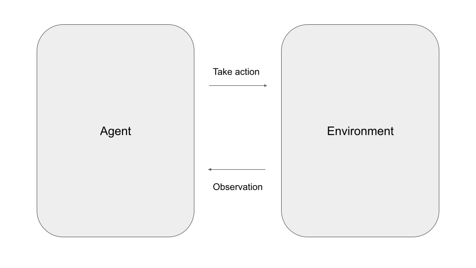
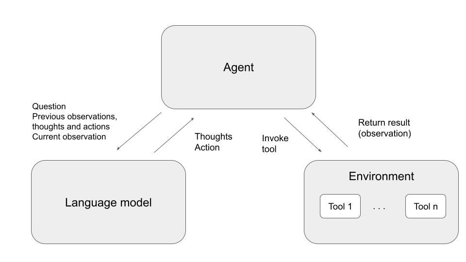
Other than most of the models we have played with so far, T5 is a full encoder-decoder model. If you have read my previous post on transformer blocks and encoder-decoder architectures, you might remember the following high-level overview of such an architecture.

For pre-training, Google did apply a method known as masking. This works as follows. Suppose your training data contains the following sentence:

The weather report predicted heavy rain for today

If we encode this using the the encoder used for training T5, we obtain the sequence of token

[37, 1969, 934, 15439, 2437, 3412, 21, 469, 1]

Note that the last token (with ID 1) is the end-of-sentence token that the tokenizer will append automatically to our input. We then select a few token in the sentence randomly and replace each of them with one of 100 special token called extra_id_NN, where NN is a number between 0 and 99. These token have IDs ranging from 32000 to 32099, where 32099 is extra token 0 and 32000 is extra token 99. After applying this procedure known as masking our sentence could look as follows

The weather report predicted heavy <extra_id_0> for today

or

[37, 1969, 934, 15439, 2437, 32099, 21, 469, 1]

We now train the decoder to output a list of the extra token used, followed by the masked word. So in our case, the target sequence for the decoder would be

<extra_id_0> rain

or, again including the end-of-sentence token

[32099, 3412, 1]

In other words, we ask our model to guess the word that has been replaced by the mask (this will remind you of the word2vec algorithm that I have presented in a previous post). To train the combination of encoder and decoder to reach that objective, we can again apply teacher forcing. For that purpose, we shift the labels to the right by one and append a special token called the decoder start token to the left (which, by the way, is identical to the padding token 0 in this case). So the input to the decoder is

[0, 32099, 3412]

We then can calculate the cross-entropy loss between the decoder output and the labels above and apply gradient descent as usual. I have put together a notebook for this post that walks you through an example and that you can also run on Google Colab as usual.

Pre-training using masking was the first stage in training T5. In a second stage, the model was fine-tuned on a set of downstream tasks. Examples for these tasks include translation, summarization, question answering and reasoning. For each task, the folks at Google defined a special format in which the model received the inputs and in which the output was expected. For translation, for instance, the task started with

“translate English to German: “

followed by the sentence to be translated, and the model was trained to reply with the correct translation. Another example is MNLI, which is a set of pairs of premise and hypothesis, and the model is supposed to answert with one word indicating whether a premise implies the hypothesis, is a contradiction to it or is neutral towards the hypothesis. In this case, the input is a sentence formatted as

“mnli premise: … premise goes here… hypothesis: … hypothesis goes here

and the model is expected to answer with one of the three words “entailment”, “contradiction” or “neutral”. So all tasks are presented to the model as pure text and the outcome is expected to be pure text. My notebook contains a few examples of how this works.

From T5 to FLAN-T5

After the pre-training using masking and the fine-tuning, T5 is already a rather powerful model, but still is sometimes not able to deduce the correct task to perform. In the notebook for this post, I hit upon a very illustrative example. If we feed the sentence

Please answer the following question: what is the boiling temperature of water?

into the model, it will not reply with the actual boiling point of water. Instead, it will fall back to one of the tasks it has been trained on and will actually translate this to German instead of answering the question.

This is where instruction fine-tuning [2] comes into play. To teach the model to recognize instructions as such and to follow them, the T5 model was trained on a large number of additional tasks, phrased in natural language.

To obtain a larger number of tasks from the given dataset, the authors applied different templates to each task. If, for instance, we are given an MNLI task with a hypothesis H and a premise P, we could present this in several ways to the model, i.e. according to several templates. We could, for instance, turn the data point into natural language using the template

“Premise: P. Hypothesis: H. Does the premise entail the hypothesis?”

Or we could phrase this as

Based on the premise P, can we conclude that the hypothesis H is true?

By combining every data point from the used data set with a certain number of templates, a large dataset for the fine-tuning was obtained, and the model learned to deal with many different instructions referring to the same type of task, which hopefully would enable the model to infer the correct tasks for an unseen template at test time. As Google published the code to generate the data, you can take a look at the templates here.

Also note that the data contains some CoT (chain-of-thought) prompting, i.e. some of the instruction templates for reasoning tasks include phrases like “apply reasoning step-by-step” to prepare the model for later chain-of-thought prompting.

In the example in my notebook, the smallest FLAN-T5 model (i.e. T5 after this additional fine-tuning procedure) did at least recognize that the input is a question, but the reply (“a vapor”) is still not what we want. The large model does in fact reply with the correct answer (212 F).

Instruction fine-tuning has become the de-facto standard for large language models. The InstructGPT model from which ChatGPT and GPT-4 are derived, however, did undergo an additional phase of training – reinforcement learning from human feedback. This is a bit more complex, and as many posts on this exist which unfortunately do only scratch the surface I will dive deeper into this in the next post which will also conclude this series.

References

[1] J. Wei et al., Finetuned Language Models Are Zero-Shot Learners, arXiv:2109.01652
[2] H.W. Chung et al., Scaling Instruction-Finetuned Language Models, arXiv:2210.11416
[3] C. Raffel et al., Exploring the Limits of Transfer Learning with a Unified Text-to-Text Transformer, arXiv:1910.10683

Mastering large language models – Part XIV: Huggingface transformers

In the previous post, we have completed our journey to being able to code and train a transformer-based language model from scratch. However, we have also seen that in order to obtain professional results, we need an enormous amount of resources, i.e. training data and compute power. Luckily, there are some pre-trained transformer models that we can use, be it directly for inference or as a basis for further fine-tuning. Today, we will take a look at the probably most prominent platform that exists for that purpose – the Huggingface platform.

Huggingface is a company that offers a variety of services around machine learning. In our context, we will mainly be interested in the wo of their products – the transformers library and the Huggingface hub, which is a platform to which scientists and enthusiasts can upload weights and trained models to make them available for everyone using the Huggingface transformer library.

As a starting point, let us first make sure that we have the library installed. For this post (and the entire series) I have used version 4.27.4, which you can install as usual.

pip3 install transformers==4.27.4

The recommended starting point for working with the library is a pipeline, which is essentially a container that includes everything which we typically need, most notably a tokenizer and a model. As the intention of this post, however, is to make contact with the models which we have implemented so far, we will dig a bit deeper and start directly with a model instead.

In the transformers library, pretrained models are usually downloaded from the hub and identified by name, which – by convention – is the name of the provider followed by a slash and the name of the model. Here is a short code snippet that you can execute in a notebook or in an interactive Python session which will download the weights for the 1.3 billion parameter version of the GPT-Neo model. GPT-Neo is a series of models developed and trained by EleutherAI and made available as open source, including the weights.

import transformers
import torch
model_name="EleutherAI/gpt-neo-1.3B"
model = transformers.AutoModelForCausalLM.from_pretrained(model_name)
print(model)
print(isinstance(model, torch.nn.Module))

Executing this for the first time will trigger the download of the model to ~/.cache/huggingface/hub. The entire download is roughly 5 GB MB, so this might take a second. If you want to avoid the large download, you can also use the much smaller 125m version – just change the last part of the model name accordingly. From the output, we can see that this model is a torch.nn.Module, so we can use it as any other PyTorch model.

We can also see that the model actually consists of two components, namely an instance of the class GPTNeoModel defined here and a linear layer – the so-called head – that is sitting on top of the actual transformer and, as usual, transforms between the model inner dimension which is 2048 and the one-hot encoded vocabulary. This decomposition of the full model into a core model and a task-specific head is common to most Huggingface models, as it allows us to use the same set of weights for different tasks.

Even though the model does not use the transformer blocks that are part of PyTorch, it is a decoder-only transformer model as we would expect it – there are two learned embeddings for positions and words and 24 transformer blocks consisting of self-attention and linear layers. There is a minor difference, though – every second layer in the GPT-Neo model uses local self-attention, which basically means that to calculate the attention at a given position, only keys and values within a sliding window are used, not all keys and values in the context – see the comment here.

Apart from this, our model is very close to the models that we have implemented and trained previously. We know how to sample from such a model. But before we can do this, we need to turn our attention to the second part of a pipeline, namely the tokenizer.

Obviously, a pretrained transformer model will only produce reasonable results if we use the same vocabulary and the same tokenizer for inference that we have used for training. Therefore, the Huggingface hub contains a matching tokenizer for every pretrained model. This tokenizer can be downloaded and initialized similar to what we have done for the model.

tokenizer = transformers.AutoTokenizer.from_pretrained(model_name)

Our tokenizer will contain everything that we need to convert forth and back between text and sequences of token. Specifically, the main components of a tokenizer are as follows.

First, there is method encode which accepts a text and returns a sequence of token IDs, and a method decode which conversely translates a sequence of token IDs into a text.

To convert between the string representation of a token and the ID, there are the methods convert_ids_to_tokens and convert_tokens_to_ids. In addition, the tokenizer obviously contains a copy of the vocabulary and some special token like a token that marks the end of a sentence (EOS token), the beginning of a sentence (BOS token), unknow token and so forth – this should in general match the token defined in the model config model.config

In our case, the tokenizer is an instance of the GPT2 tokenizer which in turn is derived from the PretrainedTokenizer class.

Having a tokenizer at our disposal, we can now sample from the model in exactly the same way as from our own models. There are two little details that we need to keep in mind. First, in the Huggingface world, the batch dimension is the first dimension. Second, the forward method of our model returns a dictionary in which the logits are stored under a key with the same name. Also, the context size is part of the model config and called max_position_embeddings. Thus our sampling method looks as follows, assuming that we have a method do_p_sampling that draws from a distribution p.

def predict(model, prompt, length, tokenizer, temperature = 0.7,  p_val = 0.95):
    model.eval()
    with torch.no_grad():
        sample = []
        device = next(model.parameters()).device
        #
        # Turn prompt into sequence of token IDs
        # 
        encoded_prompt  = tokenizer.encode(prompt)        
        encoded_sample = encoded_prompt
        encoded_prompt = torch.tensor(encoded_prompt, dtype = torch.long).unsqueeze(dim = 0)
        with torch.no_grad():
            out = model(encoded_prompt.to(device)).logits # shape B x L x V
            while (len(encoded_sample) < length):
                #
                # Sample next character from last output. Note that we need to remove the
                # batch dimension to obtain shape (L, V) and take the last element only
                #
                p = torch.nn.functional.softmax(out[0, -1, :] / temperature, dim = -1)
                #
                # Sample new index and append to encoded sample
                #
                encoded_sample.append(do_p_sampling(p, p_val))
                #
                # Feed new sequence
                #
                input = torch.tensor(encoded_sample[-model.config.max_position_embeddings:], dtype=torch.long)
                input = torch.unsqueeze(input, dim = 0)
                out = model(input.to(device)).logits
                print(tokenizer.decode(encoded_sample))

        return tokenizer.decode(encoded_sample)

This works, but it is awfully slow, even on a GPU. There is a reason for that, which is similar to what we have observed when sampling from an LSTM.

Suppose that our prompt has length L, and that we have already sampled the first token after the prompt, so that our full sample now has length L + 1. We now want to sample the next token. For that purpose, we only need the logits at position L + 1, so it might be tempting to feed only token L + 1 into our model. Let us quickly recall why this does not work.

To derive the output at position L + 1, each attention block will run the attention value at position L + 1 (which is a tensor of shape B x V) through the feed-forward network. If q denotes the query at position L + 1, this attention value is given by

\frac{1}{\sqrt{d}} \sum_{i=0}^{L} (q \cdot k_i) v_i

So we see that we need all keys and values to calculate the attention – which is not surprising, as this is the way how the model takes the context into account – but the query is only needed for position L + 1 (which is index 0, as we use zero-based indexing). Put differently, the only reason why we need to feed the previously generated token again and again into the model is that we need to key and value pairs from the past.

This hints at an opportunity to speed up inference – we could try to cache these values. To realize this, the Huggingface model returns the keys and values of all layers as an item past_key_values in the output and allows us to provide this as an additional argument to the next call. Thus instead of passing the full tensor of input IDs of length L + 1, we can as well pass only the last value, i.e. the ID of the currently last token, plus in addition the key value pairs from the previous call. Here is the updated sampling function.

def predict(model, prompt, length, tokenizer, temperature = 0.7,  p_val = 0.95):
    model.eval()
    with torch.no_grad():
        sample = []
        device = next(model.parameters()).device
        #
        # Turn prompt into sequence of token IDs
        # 
        encoded_prompt  = tokenizer.encode(prompt)        
        encoded_sample = encoded_prompt
        input_ids = torch.tensor(encoded_prompt, dtype = torch.long).unsqueeze(dim = 0)
        with torch.no_grad():
            #
            # First forward pass- use full prompt
            #
            out = model(input_ids = input_ids.to(device))
            logits = out.logits[:, -1, :] # shape B x V
            past_key_values = out.past_key_values
            while (len(encoded_sample) < length):
                #
                # Sample next character from last output
                #
                p = torch.nn.functional.softmax(logits[0, :] / temperature, dim = -1)
                #
                # Sample new index and append to encoded sample
                #
                idx = do_p_sampling(p, p_val)
                encoded_sample.append(idx)
                #
                # Feed new token and old keys and values
                #
                input_ids = torch.tensor(idx).unsqueeze(dim = 0)
                out = model(input_ids = input_ids.to(device), past_key_values = past_key_values)
                logits = out.logits
                past_key_values = out.past_key_values
                print(tokenizer.decode(encoded_sample))

        return tokenizer.decode(encoded_sample)

This should be significantly faster and provide a decent performance even on a CPU – when running this, you will also realize that the first pass that feeds the entire prompt takes some time, but all subsequent passes are much faster.

That closes our post for today. We have bridged the gap between the models that we have implemented and trained so far and the – much more advanced – models on the Huggingface hub and have convinced ourselves that even though these models are of course much larger and more powerful, their architecture is the same as for our models, and we can use them in the same way. I encourage you to play with a few other models which can be sampled from in exactly the same way, like the Pythia models from EleutherAI or the gpt2-medium and gpt2-large versions of the GPT model that can all be found on the Huggingface hub – you can use the code snippets from this post or my notebook as a starting point.

In the next post, we will use the popular Streamlit platform to implement a simple ChatBot backed by a Huggingface model.

Autonomous agents and LLMs: AutoGPT, Langchain and all that

Over the last couple of months, a usage pattern for large language models that leverages the model for decision making has become popular in the LLM community. Today, we will take a closer look at how this approach is implemented in two frameworks – Langchain and AutoGPT.

One of the most common traditional use cases in the field of artificial intelligence is to implement an agent that operates autonomously in an environment to achieve a goal. Suppose, for instance, that you want to implement an autonomous agent for banking that is integrated into an online banking platform. This agent would communicate with an environment, consisting of the end user, but maybe also backend systems of the bank that would allow it to gather information, for instance on account balances, and to trigger transactions. The goal of the agent would be to complete a customer request.

In a more abstract setting, an agent operates in discrete time steps. At each time step, it receives an observation – which, in the example above, could be a user input or the result of a call into the backend system – and can decide to take one out of a list of available actions, like making a new request to a backend system or completing the conversation with the end user – a formalism that you will have seen before if you have ever studied reinforcement learning. So the task of the agent is to select the next action, depending on the current and potentially on previous observations.

Obviously, there are many different possibilities to implement an agent – and, maybe not surprisingly, one approach that has been applied successfully in the recent past is to use a large language model as the brain of our agent. The idea behind this approach is to feed the observations, encoded as plain text, into the model at each step and to ask the model for the next action to take.

In practice, this can be done using few-shot learning, i.e. we generate a prompt for our model that consists of a few examples that inform the model about the format that we expect and the possible actions, and then add the last actual observation as a final prompt. To allow our model to take all previous observations into account, we would always include the full trajectory of observations and actions into the model.

In this paper, an approach termed ReACT (Reasoning and acting) has been proposed to orchestrate a large language model for decision making. In this framework, the environment is modelled as a set of tools that the agent can utilize. In the original paper, there are actually three tools corresponding to three different actions that the agent can take. First, it can retrieve a summary from Wikipedia. Second, it can lookup details on the Wikipedia page to which it has navigated with the first action, and finally it can complete the task and return the final result.

In each step, the agent now asks the model what action it should take next. It then runs one of the available tools to execute the action and adds the result as new observation to the next prompt that it sends to the model. To improve the quality of the results, a prompt engineering technique known as chain-of-thought prompting (CoT) is used, which basically means that the prompt contains an instruction for the model to spell out its thoughts, i.e. the rationale for the proposed action. Thus each prompt consists of the original question to be answered and the full history of thoughts, actions and observations.

Here is an example generated by the Langchain implementation of an agent following the ReACT pattern. For a better understanding, I have marked the output of the model in italic.

Question: Out of the following three countries, only two are direct neighbors of France: Germany, Spain, Poland. Please name the country in the list which is not a neighbor of France
Thought: I need to search France, find its neighbors, then find the country in the list which is not a neighbor of France
Observation: France, officially the French republic, is a country located primarily … (long summary of the Wikipedia artice on France)
Thought: France has neighbors such as Germany, Spain, Belgium, Luxemburg, Switzerland, Italy, Monaco, Andorra and the United Kingdom. So the country in the list which is not a neighbor of France is Poland.
Action: Finish[Poland]

To encourage the model to follow this pattern and to use only the allowed actions, the Langchain implementation uses few-shot learning, i.e. the prompt contains a few examples that follows this scheme (you can find these examples here, these are actually the examples cited in the original paper). So the full prompt consists of the few-shot examples, followed by the question at hand and the full sequence of observations, thoughts and actions generated so far.

Let us take a short look at the implementation in Langchain. These notes have been compiled using version 0.202. As the toolset seems to be evolving quickly, some of this might be outdated when you read this post, but I am confident that the basic ideas will remain.

First, Langchain distinguishes between an agent which is the entity talking to the language model, and the agent executor which talks to the agent and runs the tools.

The AgentExecutor class implements the main loop indicated in the diagram above. In each iteration, the method _take_next_step first invokes the agent, which will in turn assemble a prompt as explained above and generate a response from the language model. The output is then parsed and returned as an AgentAction which also contains the thought that the model has emitted. Then, the tool which corresponds to the action is executed and its output is returned along with the selected action.

Back in the main loop, we first test whether the action is an instance of the special type AgentFinish which indicates that the task is completed and we should exit the main loop. If not, we append the new tuple consisting of thought, action and observation to the history and run the next iteration of the loop. The code is actually quite readable, and I highly recommend to clone the repository and spend a few minutes reading through it.

Let us now compare this to what AutoGPT is doing. In its essence, AutoGPT uses the same pattern, but there are a few notable differences (again, AutoGPT seems to be under heavy development, at the time of writing, version 0.4.0 is the stable version and this is the version that I have used).

Similar to the ReACT agent in Langchain, AutoGPT implements an agent that interacts with an LLM and a set of tools – called commands in AutoGPT – inside a main loop. In each iteration, the agent communicates with the AI by invoking the function chat_with_ai. This function assembles a prompt and generates a reply, using the OpenAI API in the background to talk to the selected model. Then, the next action is determined based on the output of the model and executed (in the default settings, the user is asked to confirm this action before running it). Finally the results are added to the history and the next iteration starts.

The first difference compared to the ReACT agent in Langchain is how the prompt is structured. The prompt used by AutoGPT consists of three sections. First, there is a system prompt which defines a persona, i.e. it instructs the model to embody an agent aiming to achieve a certain set of goals (which are actually generated via a separate invocation of the model initially and saved in a file for later runs) and contains further instructions on the model. In particular, the system prompt instructs the model to produce output in JSON format as indicated below.

{
    "thoughts": {
        "text": "thought",
        "reasoning": "reasoning",
        "plan": "- short bulleted- list that conveys- long-term plan",
        "criticism": "constructive self-criticism",
        "speak": "thoughts summary to say to user"
    },
    "command": {
        "name": "command name",
        "args": {
            "arg name": "value"
        }
    }
} 

This is not only much more structured than the simple scheme used in the ReACT agent, but also asks the model to express its thoughts in a specific way. The model is asked to provide additional reasoning, to maintain a long-term plan as opposed to simply deciding on the next action to take and to perform self-criticism. Note that in contrast to ReACT, this is pure zero-shot learning, i.e. no examples are provided.

After the system prompt, the AutoGPT prompt contains the conversation history and finally there is a trigger prompt which is simply hardcoded to be “Determine exactly one command to use, and respond using the JSON schema specified previously:“.

Apart from the much more complex prompt using personas and a more sophisticated chain-of-thought prompting, a second difference is the implementation of an additional memory. The idea behind this is that for longer conversations, we will soon reach a point where the full history does not fit into the context any more (or it does, but we do not want to do this as the cost charged for the OpenAI API depends on the number of token). To solve this, AutoGPT adds a memory implemented by some external data store (at the time of writing, the memory system of AutoGPT is undergoing a major rewrite, so what follows is based on an analysis of earlier versions and a few assumptions).

The memory is used in two different places. First, when an iteration has been completed, an embedding vector is calculated for the results of the step, i.e. the reply of the model and the result of the executed command. The result is then stored in an external datastore, which can be as simple as a file on the local file system, but can also be a cache like Redis, and indexed using the embedding.

When an iteration is started, the agent uses an embedding calculated from the last few messages in the conversation to look up the most relevant data in memory, i.e. the results of previous iterations that have the most similar embeddings. These results are then added to the prompt, which gives the model the ability to remember previous outcomes and reuse them in a way not limited by the length of the prompt. This approach of enriching the prompt with relevant information obtained via a semantic search is sometimes called retrieval augmentation – note however that in this case, the information in the data store has been generated by model and agent, while retrieval augmentation usually leverages pre-collected data.

Finally, the AutoGPT agent can choose from a much larger variety of tools (i.e. commands in the AutoGPT terminology) than the simple ReACT agent which only had access to Wikipedia. On the master branch, there are currently commands to run arbitrary Python code, to read and write files, to clone GitHub repository, to invoke other AIs like DALL-E to generate images, to search Google or to even browse the web using Selenium. AutoGPT can also use Elevenlabs API to convert model output to speech.

AutoGPT and ReACT are not the only shows in town – there is for instance BabyAGI that lets several agents work on a list of tasks which are constantly processed, re-prioritized and amended. Similarly, HuggingGPT [7] initially creates a task list that is then processed, instead of deciding on the next action step by step (AutoGPT is an interesting mix between these approaches, as it has a concrete action for the next step, but maintains a global plan as part of its thoughts). It is more than likely that we will see a rapid development of similar approaches over the next couple of months. However, when you spend some time with these tools, you might have realized that this approach comes with a few challenges (see also the HuggingGPT paper [7] for a discussion).

First, there is the matter of cost. Currently, OpenAI charges 6 cent per 1K token for its largest GPT-4 model (and this is only the input token). If you consume the full 32K context size, this will already be 2$ per turn, so if you let AutoGPT run fully autonomously, it could easily spend an amount that hurts in a comparatively short time.

Second, if the model starts to hallucinate or to repeat itself, we can easily follow a trajectory of actions that takes us nowhere or end up in a loop. This has already been observed in the original ReACT paper, and I had a similar experience with AutoGPT – asking for a list of places in France to visit, the agent started to gather more and more detailed information and completely missed the point where I would have been happy to get an answer compiled out of the information that it already had.

Last but not least the use of autonomous agents that execute Python code, access files on your local system, browse the web using your browser and your IP address or even send mails and trigger transactions on your behalf can soon turn into a nightmare in terms of security, especially given that the output of commands ends up in the next prompt (yes, there is something like a prompt injection, see [8] and [9]). Clearly, a set of precautions is needed to make sure that the model does not perform harmful or dangerous actions ([6] provides an example where AutoGPT was starting to install updated SSL certificates to solve a task that a straight-forward web scraping could have solved as well).

Still, despite of all this, autonomous agents built on top of large language models are clearly a very promising approach and I expect to see more powerful, but also more stable and reliable solutions being pushed into the community very soon. Unitl then, you might want to read some of the references that I have assembled that discuss advanced prompting techniques and autonomous agents in more details.

References:

[1] S. Yao et al., ReAct: Synergizing Reasoning and Acting in Language Models, arXiv:2210.03629
[2] Prompt Engineering guide at https://www.promptingguide.ai/
[3] N. Shinn et al., Reflexion: Language Agents with Verbal Reinforcement Learning, arXiv:2303.11366
[4] L. Wang et al., Plan-and-Solve Prompting: Improving Zero-Shot Chain-of-Thought Reasoning by Large Language Models, arXiv:2305.04091
[5] Ask Marvin – integrate AI into your codebase
[6] https://www.linkedin.com/pulse/auto-gpt-promise-versus-reality-rick-molony – an interesting experience with AutoGPT
[7] Y. Shen, HuggingGPT: Solving AI Tasks with ChatGPT and its Friends in Hugging Face, arXiv:2303.17580 – also known as JARVIS
[8] C. Anderson, https://www.linkedin.com/pulse/newly-discovered-prompt-injection-tactic-threatens-large-anderson/
[9] OWASP Top 10 for LLM Security

Running and using Go-Ethereum

Most of the time, we have been using the Brownie development environment for our tests so far, and with it the Ganache Ethereum client that Brownie runs behind the scenes. For some applications, it is useful to have other clients at our disposal. The Go-Ethereum client (geth) is the most commonly used client at the time of writing, and today we take a slightly more detailed look at how to run and configure it.

Getting started

We have already installed the geth binary in a previous post, so I assume that the geth binary is still on your path. However, geth is evolving quickly – when I started this series, I used version 1.10.6, but in the meantime, 1.10.8 has been released which contains an important bugfix (for this vulnerability which we have analyzed in depth in a previous post ), so let us use this going forward. So please head over to the download page, get the archive for version 1.10.8 for your platform (here is the link for Linux AMD64), extract the archive, copy the geth binary to a location on your path and make it executable.

Geth stores blockchain data and a keystore in a data directory which can be specified via a command line flag. We will use ~/.ethereum, and it is easier to follow along if you start over with a clean setup, so if you have used geth before, you might want to delete the contents of the data directory before proceeding. To actually start the client, we can then use the command

geth --dev \
     --datadir=$HOME/.ethereum \
     --http \
     --http.corsdomain="*" \
     --http.vhosts="*" \
     --http.addr="0.0.0.0" \
     --http.api="eth,web3"

For the sake of convenience, I have put that command into a script in the tools directory of my repository, so if you have a clone of this directory, you could as well run ./tools/run_geth. Let us go through the individual flags that we have used and try to understand what they imply.

First, there is the dev flag. If you start geth with this flag, the client will actually not try to connect to any peers. Instead, it will create a local blockchain, with a genesis block which is created on the fly (here). In addition, geth will create a so-called developer account (or re-use an existing one). This account shows up at several places. It will be the first account in the keystore managed by geth and therefore the first account that the API method eth_accounts will return. This account (or rather the associated address) will also be used as the etherbase, i.e. as the address to which mined Ether will be credited. Finally, the genesis contains an allocation of 2256 – 9 Wei (the genesis block will also contain allocations for the nine pre-compiled contracts).

The next flag is the data directory, which we have already discussed. The following couple of flags are more interesting and configure the HTTP endpoint. Geth offers APIs over three different channels – HTTP, WebSockets (WS) and a local Unix domain socket (IPC). Whereas the IPC endpoint is enabled by default, the other two are disabled by default, and the http flag enables the HTTP endpoint.

The next three flags are important, as they determine who is allowed to access this API. First, http.address is the address on which the client will be listening. By default, this is the local host (i.e. 127.0.0.1), which implies that the client cannot be reached from the outside world. Especially, this will not work if you run geth inside a docker container or virtual machine. Specifying 0.0.0.0 as in the example above allows everybody on the local network to connect to your client – this is of course not a particularly secure setup, so modify this if you are not located on a secure and private network.

In addition, geth also uses the concept of a virtual host to validate requests. Recall that RFC7320 defines the HTTP header field Host which is typically used to allow different domains to be served by one web server running on one IP address only. This field is added by web browsers to requests that are the result of a navigation, but also the requests generated by JavaScript code running in the browser. When serving an incoming request, geth will validate the content of this header field against a list configured via the http.vhosts flag. This flag defaults to “localhost”. Thus, if you want to serve requests from outside, maybe from a web browser running on a different machine in your local network, you have to set this flag, either to the domain name of your server or using the wildcard “*” to accept incoming requests regardless of the value of the host header.

Finally, there is the CORS domain flag http.corsdomain. CORS is the abbreviation for cross-origin request surgery and refers to an attack which tries to access a server from JavaScript code loaded from a different domain. To prevent this sort of attack, browsers ask a server upfront before sending such a request whether the server will accept the request by submitting a so-called pre-flight request. When we develop our frontend later on, we will need to make sure that this pre-flight request is successful, so we need to include the domain from which we will load our JavaScript code to the list that we configure here, or, alternatively, also use a wildcard here. If you want to learn more about CORS, you might want to read this documentation on the Mozilla developer network.

The last flag that we use determines which of the APIs that geth offers will be made available via the HTTP endpoint. The most important API is the eth API, which contains all the methods that we need to submit and read transactions, get blocks or interact with smart contracts. In addition, it might be helpful to enable the debug API, which we will use a bit later when tracing transactions. There are also a few APIs which you almost never want to make available over the network like the personal API which allows you to access the accounts maintained by the client, or the admin API.

Using the geth console

We have just mentioned that there are some APIs which you would typically not want to make accessible via the API. Instead, you usually access these APIs via the IPC endpoint and the geth console. This is a JavaScript-based interactive console that allows you to invoke API methods and thus interact with a running geth client. To start the console, make sure that the geth client is running, open a separate terminal window and enter

geth attach ~/.ethereum/geth.ipc

Note that the second argument is the Unix domain socket that geth will create in its data directory. To see how the console works, let us play a bit with accounts. At the prompt, enter the following commands.

eth.blockNumber
eth.accounts
eth.getBlockByNumber(0)

The first command will return the block number for the block at the head of the chain. Currently, this is zero – we only have the genesis block, no other blocks. The second command displays the list of accounts managed by the node. You should see one account, which is the developer accounts mentioned earlier. The third command displays the genesis block, and you will see that the extra data also contains the developer account.

The accounts managed by the node can be controlled using the personal API. An important functionality of this API is that accounts can be locked, so that they can no longer be used. As an example, let us try to lock the developer account.

dev = eth.accounts[0]
personal.lockAccount(dev)

Unlocking the account again is a bit tricky, as this is not allowed while the HTTP endpoint is being served. So to unlock again, you will have to shutdown geth, start it again without the HTTP flags, attach again and execute the command

personal.unlockAccount(eth.accounts[0], "")

Note the second argument – this is the password that has been used to lock the account (at startup, geth creates the development account with an empty passphrase, alternatively a passphrase can be supplied using the —password command line flag).

Finally, let us see how to use the console to create additional accounts and transfer Ether to them.

dev = eth.accounts[0]
alice = personal.newAccount("secret")
value = web3.toWei(1, "ether")
gas = 21000
gasPrice = web3.toWei(1, "gwei")
txn = {
        from: dev, 
        to: alice, 
        gas: gas, 
        gasPrice: gasPrice, 
        value: value
}
hash = eth.sendTransaction(txn)
eth.getTransactionReceipt(hash)
eth.getBalance(alice)

You could now proceed like this and set up a couple of accounts, equipped with Ether, for testing purposes. To simplify this procedure, I have provided a script that sets up several test accounts – if you have cloned the repository, simply run it by typing

python3 tools/GethSetup.py

Geth and Brownie

What about Brownie? Do we have to say good-bye to our good old friend Brownie if we choose to work with geth? Fortunately the answer is no – Brownie is in fact smart enough and will automatically detect a running geth (in fact, a running Ethereum client) when it is started and use it instead of launching Ganache. Let us try this. Make sure that geth is running and start Brownie as usual.

brownie console

At this point, it is important that we have enabled the web3 API when starting geth, as Brownie uses the method web3_clientVersion to verify connectivity at startup. If everything works, Brownie will spit out a warning that the blockchain that it has detected has a non-zero length and greet you with the usual prompt.

Great, so let us transfer some Ether to a new account as we have done it before from the console to see that everything works.

dev = accounts[0]
bob = accounts.add()
dev.transfer(to=bob, amount=web3.toWei(1, "ether"))

Hmm…this does not look good. It appears that Brownie has created a transaction and sent it, but is now waiting for the receipt and does not receive it. To understand the problem, let us switch again to a different terminal and start the geth console again. At the console prompt, inspect the pending transactions by running

txpool

The output should show you that there is one pending transaction (which you can also inspect by using eth.getTransaction) which is not included in a block yet. If you look at this transaction for a second, you will find that there are two things that look suspicious. First, the gas price for the transaction is zero. Second, the gas limit is incredibly high. If you inspect the last block that has been mined, you will find that the gas limit is exactly the gas limit of the last block that has been mined successfully.

Why is this a problem? The gas limit for a new block is determined by geth aiming at a certain target value. At the moment, this target value is lower than the gas limit of the genesis block, meaning that geth will try to decrease the gas limit with each new block (the exact algorithm is here). Thus the gas limit for the new block that the miner tries to assemble is lower than that for the previous one and therefore lower than the gas limit of our transaction, so that the transaction will not fit into the block and the miner will ignore it.

Let us try to fix this. First, we need to replace our pending transaction. The easiest way to do this is to use the geth console. What we need to do is to get the transaction from the pool of pending transactions, correct the gas limit and increase the gas price, so that the miner will pick up this transaction instead of the previous one. We also set the value to zero, so that the transaction will effectively be cancelled.

txn = eth.pendingTransactions[0]
txn.gas = eth.estimateGas(txn)
txn.gasPrice = web3.toWei(1, "gwei")
txn.value = 0
eth.sendTransaction(txn)

Note that we did not change the nonce, so our transaction replaces the pending one. After a few seconds, Brownie should note that the transaction has been dropped and stop waiting for a receipt.

The reason for our problem is related to the way how Brownie determines the gas limit and gas price to be used for a transaction. When a transaction is created, Brownie tries to figure out a gas limit and gas price from the network configuration. For the gas limit, the default setting is “max”, which instructs Brownie to use the block gas limit of the latest blocks (which will be cached for one hour). For the gas price, the default is zero. To make Brownie work with geth, we need to adjust both settings. In the console, enter

network.gas_limit("auto")
network.gas_price("auto")

When you now repeat the commands above to transfer Ether, the transaction should go through. For versions of Brownie newer than version 1.15.2, however, you will receive an error message saying that the sleep method is not implemented by geth. The transaction will still work (the error comes from this line of the code which is executed in a separate thread initiated here), so the error message is only annoying, however you might want to downgrade to version 1.15.2 if you plan to work with Brownie and geth more often (it appears that the problem was introduced with this commit).

Note that the settings for the gas price and the gas limit that we have made enough will be lost when we restart Brownie. In order to make these changes permanent, you can add them to the configuration file for Brownie. Specifically, Brownie will, upon startup, load configuration data from a file called brownie-config.yaml. To set the gas price and the gas limit, create such a file with the following content

networks:
    default: development
    development:
        gas_limit: auto
        gas_price: auto

Here we adjust the configuration for the network development which we also declare as the default network and set the gas limit and the gas price to “auto”, instructing Brownie to determine a good approximation at runtime.

This closes our post for today. We have learned how to run geth in a local development environment, discussed the most important configuration options and seen how we can still use Brownie to work with transactions and contracts. In the next post, we will start to design and build our NFT wallet application and first try to understand the overall architecture.

Implementing and testing an ERC721 contract

In the previous posts, we have discussed the ERC721 standard and how metadata and the actual asset behind a token are stored. With this, we have all the ingredients in place to tackle the actual implementation. Today, I will show you how an NFT contract can be implemented in Solidity and how to deploy and test a contract using Brownie. The code for this post can be found here.

Data structures

As for our sample implementation of an ERC20 contract, let us again start by discussing the data structures that we will need. First, we need a mapping from token ID to the current owner. In Solidity, this would look as follows.

mapping (uint256 => address) private _ownerOf;

Note that we declare this structure as private. This does not affect the functionality, but for a public data structure, Solidity would create a getter function which blows up the contract size and thus makes deployment more expensive. So it is a good practice to avoid public data structures unless you really need this.

Now mappings in Solidity have a few interesting properties. In contrast to programming languages like Java or Python, Solidity does not offer a way to enumerate all elements of a mapping – and even if it did, it would be dangerous to use this, as loops like this can increase the gas usage of your contract up to the point where the block limit is reached, rendering it unusable. Thus we cannot simply calculate the balance of an owner by going through all elements of the above mapping and filtering for a specific owner. Instead, we maintain a second data structure that only tracks balances.

mapping (address => uint256) private _balances;

Whenever we transfer a token, we also need to update this mapping to make sure that it is in sync with the first data structure.

We also need a few additional mappings to track approvals and operators. For approvals, we again need to know which address is an approved recipient for a specific token ID, thus we need a mapping from token ID to address. For operators, the situation is a bit more complicated. We set up an operator for a specific address (the address on behalf of which the operator can act), and there can be more than one operator for a given address. Thus, we need a mapping that assigns to each address another mapping which in turn maps addresses to boolean values, where True indicates that this address is an operator for the address in the first mapping.

/// Keep track of approvals per tokenID
mapping (uint256 => address) private _approvals; 

/// Keep track of operators
 mapping (address => mapping(address => bool)) private _isOperatorFor;

Thus the sender of a message is an operator for an address owner if and only if _isOperatorFor[owner][msg.sender] is true, and the sender of a message is authorized to withdraw a token if and only if _approvals[tokenID] === msg.sender.

Burning and minting a token is now straightforward. To mint, we first check that the token ID does not yet exist. We then increase the balance of the contract owner by one and set the owner of the newly minted token to the contract owner, before finally emitting an event. To burn, we reverse this process – we set the current owner to the zero address and decrease the balance of the current owner. We also reset all approvals for this token. Note that in our implementation, the contract owner can burn all token, regardless of the current owner. This is useful for testing, but of course you would not want to do this in production – as a token owner, you would probably not be very amused to see that the contract owner simply burns all your precious token. As an aside, if you really want to fire up your own token in production, you would probably want to take a look at one of the available audited and thoroughly tested sample implementations, for instance by the folks at OpenZeppelin.

Modifiers

The methods to approve and make transfers are rather straightforward (with the exception of a safe transfer that we will discuss separately in a second). If you look at the code, however, you will spot a Solidity feature that we have not used before – modifiers. Essentially, a modifier is what Java programmers might know as an aspect – a piece of code that wraps around a function and is invoked before and after a function in your contract. Specifically, if you define a modifier and add this modifier to your function, the execution of the function will start off by running the modifier until the compiler hits upon the special symbol _ in the modifier source code. At this point, the code of the actual function will be executed, and if the function completes, execution continues in the modifier again. Similar to aspects, modifiers are useful for validations that need to be done more than once. Here is an example.

/// Modifier to check that a token ID is valid
modifier isValidToken(uint256 _tokenID) {
    require(_ownerOf[_tokenID] != address(0), _invalidTokenID);
    _;
}

/// Actual function
function ownerOf(uint256 tokenID) external view isValidToken(tokenID) returns (address)  {
    return _ownerOf[tokenID];
}

Here, we declare a modifier isValidToken and add it to the function ownerOf. If now ownerOf is called, the code in isValidToken is run first and verifies the token ID. If the ID is valid, the actual function is executed, if not, we revert with an error.

Safe transfers and the code size

Another Solidity feature that we have not yet seen before is used in the function _isContract. This function is invoked when a safe transfer is requested. Recall from the standard that a safe transfer needs to check whether the recipient is a smart contract and if yes, tries to invoke its onERC721Received method. Unfortunately, Solidity does not offer an operation to figure out whether an address is the address of a smart contract. We therefore need to use inline assembly to be able to directly run the EXTCODESIZE opcode. This opcode returns the size of the code of a given address. If this is different from zero, we know that the recipient is a smart contract.

Note that if, however, the code size is zero, the recipient might in fact still be a contract. To see why, suppose that a contract calls our NFT contract within its constructor. As the code is copied to its final location after the constructor has executed, the code size is still zero at this point. In fact, there is no better and fully reliable way to figure out whether an address is that of a smart contract in all cases, and even the ERC-721 specification itself states that the check for the onERC721Received method should be done if the code size is different from zero, accepting this remaining uncertainty.

Inline assembly is fully documented here. The code inside the assembly block is actually what is known as Yul – an intermediate, low-level language used by Solidity. Within the assembly code, you can access local variables, and you can use most EVM opcodes directly. Yul also offers loops, switches and some other high-level constructs, but we do not need any of this in your simple example.

Once we have the code size and know that our recipient is a smart contract, we have to call its onERC721Received method. The easiest way to do this in Solidity is to use an interface. As in other programming languages, an interface simply declares the methods of a contract, without providing an implementation. Interfaces cannot be instantiated directly. Given an address, however, we can convert this address to an instance of an interface, as in our example.

interface ERC721TokenReceiver
{
  function onERC721Received(address, address, uint256, bytes calldata) external returns(bytes4);
}

/// Once we have this, we can access a contract with this interface at 
/// address to
ERC721TokenReceiver erc721Receiver = ERC721TokenReceiver(to);
bytes4 retval = erc721Receiver.onERC721Received(operator, from, tokenID, data);

Here, we have an address to and assume that at this address, a contract implementing our interface is residing. We then convert this address to an instance of a contract implementing this interface, and can then access its methods.

Note that this is a pure compile-time feature – this code will not actually create a contract at the address, but will simply assume that a contract with that interface is present at the target location. Of course, we can, at compile time, not know whether this is really the case. The compiler can, however, prepare a call with the correct function signature, and if this method is not implemented, we will most likely end up in the fallback function of the target contract. This is the reason why we also have to check the return value, as the fallback function might of course execute successfully even if the target contract does not implement onERC721Received.

Implementing the token URI method

The last part of the code which is not fully straightforward is the generation of the token URI. Recall that this is in fact the location of the token metadata for a given token ID. Most NFT contracts that I have seen build this URI from a base URI followed by the token ID, and I have adapted this approach as well. The base URI is specified when we deploy the contract, i.e. as a constructor argument. However, converting the token ID into a string is a bit tricky, because Solidity does again not offer a standard way to do this. So you either have to roll your own conversion or use one of the existing implementations. I have used the code from this OpenZeppelin library to do the conversion. The code is not difficult to read – we first determine the number of digits that our number has by dividing by ten until the result is less than one (and hence zero – recall that we are dealing with integers) and then go through the digits from the left to the right and convert them individually.

Interfaces and the ERC165 standard

Our smart contract implements a couple of different interfaces – ERC-721 itself and the metadata extension. As mentioned above, interfaces are a compile-time feature. To improve type-safety at runtime, it would be nice to have a feature that allows a contract to figure out whether another contract implements a given interface. To solve this, EIP-165 has been introduced. This standard does two things.

First, it defines how a hash value can be assigned to an interface. The hash value of an interface is obtained by taking the 4-byte function selectors of each method that the interface implements and then XOR’ing these bytes. The result is a sequence of four bytes.

Second, it defines a method that each contract should implement that can be used to inquire whether a contract implements an interface. This method, supportsInterface, accepts the four-byte hash value of the requested interface as an argument and is supposed to return true if the interface is supported.

This can be used by a contract to check whether another contract implements a given interface. The ERC-721 standard actually mandates that a contract that implements the specification should also implement EIP-165. Our contract does this as well, and its supportsInterface method returns true if the requested interface ID is

  • 0x01ffc9a7, which corresponds to ERC-165 itself
  • 0x80ac58cd which is the hash value corresponding to ERC-721
  • 0x5b5e139f which is the hash value corresponding to the metadata extension

Testing, deploying and running our contract

Let us now discuss how we can test, deploy and run our contract. First, there is of course unit testing. If you have read my post on Brownie, the unit tests will not be much of a surprise. There are only two remarks that might be in order.

First, when writing unit tests with Brownie and using fixtures to deploy the required smart contracts, we have a choice between two different approaches. One approach would be to declare the fixtures as function scoped, so that they are run over and over again for each test case. This has the advantage that we start with a fresh copy of the contract for each test case, but is of course slow – if you run 30 unit tests, you conduct 30 deployments. Alternatively, we can declare the fixture as sessions-scoped. They will then be only executed once per test session, so that every test case uses the same instance of the contract under test. If you do this, be careful to clean up after each test case. A disadvantage of this approach, though, remains – if the execution of one test case fails, all test cases run after the failing test case will most likely fail as well because the clean up is skipped for the failed test case. Be aware of this and do not panic if all of a sudden almost all of your test cases fail (the -x switch to Brownie could be your friend if this happens, so that Brownie exits if the first test case fails).

A second remark is concerning mocks. To test a safe transfer, we need a target contract with a predictable behavior. This contract should implement the onERC721Received method, be able to return a correct or an incorrect magic value and allow us to check whether it has been called. For that purpose, I have included a mock that can be used for that purpose and which is also deployed via a fixture.

To run the unit tests that I have provided, simply clone my repository, make sure you are located in the root of the repository and run the tests via Brownie.

git clone https://github.com/christianb93/nft-bootcamp.git
cd nft-bootcamp
brownie test tests/test_NFT.py

Do not forget to first active your Python virtual environment if you have installed Brownie or any of the libraries that it requires in a virtual environment.

Once the unit tests pass, we can start the Brownie console which will, as we know, automatically compile all contracts in the contract directory. To deploy the contract, run the following commands from the Brownie console.

owner = accounts[0]
// Deploy - the constructor argument is the base URI
nft = owner.deploy(NFT, "http://localhost:8080/")

Let us now run a few tests. We will mint a token with ID 1, pick a new account, transfer the token to this account, verify that the transfer works and finally get the token URI.

alice = accounts[1]
nft._mint(1)
assert(owner == nft.ownerOf(1))
nft.transferFrom(owner, alice, 1)
assert(alice == nft.ownerOf(1))
nft.tokenURI(1)

I invite you to play around a bit with the various functions that the NFT contract offers – declare an operator, approve a transfer, or maybe test some validations. In the next few posts, we will start to work towards a more convenient way to play with our NFT – a frontend written using React and web3.js. Before we are able to work on this, however, it is helpful to expand our development environment a bit by installing a copy of geth, and this is what the next post will be about. Hope to see you there.

Basis structure of a token and the ERC20 standard

What is a token? The short answer is that a token is a smart contract that records and manages ownership in a digital currency. The long answer is in this post.

Building a digital currency – our first attempt

Suppose for a moment you wanted to issue a digital currency and were thinking about the design of the required software package. Let us suppose further that you have never heard of a blockchain before. What would you probably come up with?

First, you would somehow need to record ownerhip. In other words, you will have to store balances somewhere, and associate a balance to every participant or client in the system, represented by an account. In a traditional IT, this would imply that somewhere, you fire up a database, maybe a relational database, that has a table with one row per account holding the current balance of this account.

Next, you would need a function that allows you to query the balance, something like balanceOf, to which you pass an account and with returns the balance of this account, looking up the value in the database. And finally, you would want to make a transfer. So you would have a method transfer which the owner of an account can use to transfer a certain amount to another account. This method would of course have to verify that whoever calls it (say you expose it as an API) is the holder of the account from which the transfer is made, which could be done using certificates or digital signatures and is well possible with traditional technology. So your first design would be rather minimalistic.

This would probably work, but is not yet very powerful. Let us add a direct debit functionality, i.e. let us allow users to withdraw a pre-approved amount of money from an account. To realize this, you could come up with a couple of additional functions.

  • First, you would add a function approve() that the owner of an account can invoke to grant permission to someone else (identified again by an account) to withdraw a certain amount of currency
  • You would probably also want to store these approvals in the database and add a function approval() to read them out
  • Finally, you would add a second function – say transferFrom – to allow withdrawals

Updating your diagram, you would thus arrive at the following design for your digital currency.

This is nice, but it still has a major drawback – someone will eventually need to operate the database and the application, and could theoretically manipulate balances and allowances directly in the database, bypassing all authorizations. The same person could also try to manipulate the code, building in backdoors or hidden transfers. So this system only qualifies as an acceptable digital currency if it is embedded into a system of regulations and audits that tries to avoid these sort of manipulations.

The ERC20 token standard

Now suppose further that you are still sitting in at your desk and scratching your head, thinking about this challenge when someone walks into your office and tells you that a smart person has just invented a technology called blockchain that allows you to store data in way that makes it extremely hard to manipulate it and also allows you to store and run immutable programs called smart contracts. Chances are that this would sound like the perfect solution to you. You would dig into this new thing, write a smart contract that stores balances and approvals in its storage on the blockchain and whose methods implement the functions that appear in your design, and voila – you have implemented your first token.

Essentially, this is how a token works. A token is a smart contract that, in its storage, maintains a data structure mapping accounts to balances, and offers methods to transfer digital currency between accounts, thus realizing a digital currency on top of Ethereum. These “sub-currencies” were among the first applications of smart contracts, and attempts to standardize these contracts have already been started in 2015, shortly after the Ethereum blockchain was launched (see for instance this paper cited by the later standard). The final standard is now known as ERC20.

I strongly advise you to take a look at the standard itself, which is actually quite readable. In addition to the functions that we have already discussed, it defines a few optional methods to read token metadata (like its name, a symbol and how to display decimals), a totalSupply method that returns the total number of token emitted and events that fire when approvals are made or token are transferred. Here is an overview of the components of the standard.

Note that it is up to the implementation whether the supply of token is fixed or token can be created (“minted”) or burnt. The standard does, however, specify that an implementation should emit an event if this happens.

Coding a token in Solidity

Let us now discuss how to implement a token according to the ERC20 standard in Solidity. The code for our token can be found here. Most of it is straightforward, but there is a couple of features of the Solidity language that we have not yet come across and that require explanation.

First, let us think about the data structures that we will need. Obviously, we somehow need to store balances per account. This calls for a mapping, i.e. a set of key-value pairs, where the keys are addresses and the value for a given address is the balance of this address, i.e. the number of token owned by this address. The value can be described by an integer, say a uint256. The address is not simply a string, as Solidity has a special data type called address. So the data structure to hold the balances is declared as follows.

mapping(address => uint256) private _balances;

Mappings in Solidity are a bit special. First, there is no way to visit all elements of a map like this, i.e. there nothing like x.keys() to get a list of all keys that appear in the mapping. Solidity will also allow you to access an element of a mapping that has not been initialized, this will return the default value for the respective data type, i.e. zero in our case. Thus, logically, our mapping covers all possible addresses and assigns an initial balance zero to them.

A similar mapping can be used to track allowances. This is a mapping whose values are again mappings. The first key (the key of the top-level mapping) is the owner of the account, the second key is the address authorized to perform a transfer (called the spender) , and the value is the allowance.

mapping (address => mapping (address => uint256)) private _allowance;

The next mechanism that we have not yet seen is the constructor which will be called when the contract is deployed. We use it to initialize some variables that we will need later. First, we store the msg.sender which is one of the pre-defined variables in Solidity and is the address of the account that invoked the constructor, i.e. in our case the account that deployed the contract. Note that msg.sender refers to the address of the EOA or contract that is the immediate predecessor of the contract in the call chain. In contrast to this, tx.origin is the EOA that signed the transaction. In the constructor, we also set up the initial balance of the token owner.

The remaining methods are straightforward, with one exception – validations. Of course, we need to validate a couple of things, for instance that the balance is sufficient to make a transfer. Thus we would check a condition, and, depending on the boolean value of that condition, revert the transaction. This combination is so common that Solidity has a dedicated instruction to do this – require. This accepts a boolean expression and a string, and, if the expression evaluates to false, reverts using the string as return value. Unfortunately, it is currently not possible for an EOA to get access to the return value of a reverted transaction, as this data is not part of the transaction receipt (see EIP-658 and EIP-758 for some background on this), but this is possible if you make a call to the contract.

This raises an interesting question. In some unit tests, for instance in this one that I have written to test my token implementation, we test whether a transaction reverts by assuming that submitting a transaction raises a Python exception. For instance, the following lines

with brownie.reverts("Insufficient balance"):
    token.transfer(alice.address, value, {"from": me.address});

verify that the transfer method of our token contract actually reverts with an expected message. Now we have just seen that the message is not part of the transaction receipt – how does Brownie know? It turns out that the handling of reverted transactions in the various frameworks is a bit tricky, in this case this works because we do not provide a gas limit – I will dive a bit deeper into the mechanics of revert in a later post.

Testing the token using MetaMask

Let us now deploy and test our token. If you have not done so, clone my repository, set up a Brownie project directory, add symbolic links to the contracts and test cases and run the tests.

git clone https://github.com/christianb93/nft-bootcamp
cd nft-bootcamp
mkdir tmp
cd tmp
brownie init
cd contracts
ln ../../contracts/Token.sol .
cd ../tests
ln ../../tests/test_Token.py
cd ..
brownie test 

Assuming that the unit tests complete successfully, we can use Brownie to deploy a copy of the token as usual (or any of the alternative methods discussed in previous posts)

brownie console
me = accounts[0]
token = Token.deploy({"from": me})
token.balanceOf(me)

At this point, the entire supply of token is allocated to the contract owner. To play with MetaMask, we need two additional accounts of which we know the private keys. Let us call them Alice and Bob. Enter the following commands to create these accounts and make sure to write down their addresses and private keys. We also transfer an initial supply of 1000 token to Alice and equip Alice with some Ether to be able to make transactions.

alice = accounts.add()
alice.private_key
alice.address
bob = accounts.add()
bob.private_key
bob.address
token.transfer(alice, 1000, {"from": me})
me.transfer(alice, web3.toWei(1, "ether"))
alice.balance()

Next, we will import or keys and token into MetaMask. If you have not done this yet, go ahead and install the MetaMask extension for your browser. You will be directed to the extension store for your browser (I have been using Chrome, but Firefox should work as well). Add the extension (you might want to use a separate profile for this). Then follow the instructions to create a new wallet. Set a password to protect your wallet and save the seed phrase somewhere.

You should now see the MetaMask main screen in front of you. At the right hand side at the top of the screen, you should see a switch to select a network. Click on it and select “Localhost 8545” to connect to the – still running – instance of Ganache. Then, click on the icon next to the network selector and import the account of Alice by entering the private key. You should now see a new account (for me, this was “Account 2”) with the balance of 1 ETH.

Next, we will add the token. Click on “Add Token”, collect the contract address from brownie (token.address) and enter it. You should now see a balance of “10 MTK”. Note how MetaMask uses the decimals – Alice owns 1000 token, and we have set the decimals (the return value of token.decimals()) to two, so that MetaMask interprets the last two zeros as decimals and displays ten.

Now let us use MetaMask to make a transfer – we will send 100 token to Bob. Click on “Send” and enter the address of Bob. Now select 1 MTK (remember the decimals again). Confirm the transaction. After a few seconds, MetaMask should inform you that the transaction has been mined. You will also see that the balance of Alice in ETH has decreased slightly, as she needed to pay for the gas, and her MTK balance has been decreased. Finally, switch back to Brownie and run

token.balanceOf(bob)

to confirm that Bob is now proud owner of 100 token.

Today, we have discussed the structure of a token contract, introduced you to the ERC20 standard, presented an implementation in Solidity and verified that this contract is able to interact with the MetaMask wallet as expected. In the next post, we will discuss a few of the things that can go terribly wrong if you implement smart contracts without thinking about the potential security implications of your design decisions.

Compiling and deploying a smart contract with geth and Python

In our last post, we have been cheating a bit – I have shown you how to use the web3 Python library to access an existing smart contract, but in order to compile and deploy, we have still been relying on Brownie. Time to learn how this can be done with web3 and the Python-Solidity compiler interface as well. Today, we will also use the Go-Ethereum client for the first time. This will be a short post and the last one about development tools before we then turn our attention to token standards.

Preparations

To follow this post, there is again a couple of preparational steps. If you have read my previous posts, you might already have completed some of them, but I have decided to list them here once more, in case you are just joining us or start over with a fresh setup. First, you will have to install the web3 library (unless, of course, you have already done this before).

sudo apt-get install python3-pip python3-dev gcc
pip3 install web3

The next step is to install the Go-Ethereum (geth) client. As the client is written in Go, it comes as a single binary file, which you can simply extract from the distribution archive (which also contains the license) and copy to a location on your path. As we have already put the Brownie binary into .local/bin, I have decided to go with this as well.

cd /tmp
wget https://gethstore.blob.core.windows.net/builds/geth-linux-amd64-1.10.6-576681f2.tar.gz
gzip -d geth-linux-amd64-1.10.6-576681f2.tar.gz
tar -xvf  geth-linux-amd64-1.10.6-576681f2.tar
cp geth-linux-amd64-1.10.6-576681f2/geth ~/.local/bin/
chmod 700 ~/.local/bin/geth
export PATH=$PATH:$HOME/.local/bin

Once this has been done, it is time to start the client. We will talk more about the various options and switches in a later post, when we will actually use the client to connect to the Rinkeby testnet. For today, you can use the following command to start geth in development mode.

geth --dev --datadir=~/.ethereum --http

In this mode, geth will be listening on port 8545 of your local PC and bring up local, single-node blockchain, quite similar to Ganache. New blocks will automatically be mined as needed, regardless of the gas price of your transactions, and one account will be created which is unlocked and at the same time the beneficiary of newly mined blocks (so do not worry, you have plenty of Ether at your disposal).

Compiling the contract

Next, we need to compile the contract. Of course, this comes down to running the Solidity compiler, so we could go ahead, download the compiler and run it. To do this with Python, we could of course invoke the compiler as a subprocess and collect its output, thus effectively wrapping the compiler into a Python class. Fortunately, someone else has already done all of the hard work and created such a wrapper – the py-solc-x library (a fork of a previous library called py-solc). To install it and to instruct it to download a specific version of the compiler, run the following commands (this will install the compiler in ~/.solcx)

pip3 install py-solc-x
python3 -m solcx.install v0.8.6
~/.solcx/solc-v0.8.6 --version

If the last command spits out the correct version, the binary is installed and we are ready to use it. Let us try this out. Of course, we need a contract – we will use the Counter contract from the previous posts again. So go ahead, grab a copy of my repository and bring up an interactive Python session.

git clone https://github.com/christianb93/nft-bootcamp
cd nft-bootcamp
ipython3

How do we actually use solcx? The wrapper offers a few functions to invoke the Solidity compiler. We will use the so-called JSON input-output interface. With this approach, we need to feed a JSON structure into the compiler, which contains information like the code we want to compile and the output we want the compiler to produce, and the compiler will spit out a similar structure containing the results. The solcx package offers a function compile_standard which wraps this interface. So we need to prepare the input (consult the Solidity documentation to better understand what the individual fields mean), call the wrapper and collect the output.

import solcx
source = "contracts/Counter.sol"
file = "Counter.sol"
spec = {
        "language": "Solidity",
        "sources": {
            file: {
                "urls": [
                    source
                ]
            }
        },
        "settings": {
            "optimizer": {
               "enabled": True
            },
            "outputSelection": {
                "*": {
                    "*": [
                        "metadata", "evm.bytecode", "abi"
                    ]
                }
            }
        }
    };
out = solcx.compile_standard(spec, allow_paths=".");

The output is actually a rather complex data structures. It is a dictionary that contains the contracts created as result of the compilation as well as a reference to the source code. The contracts are again structured by source file and contract name. For each contract, we have the ABI, a structure called evm that contains the bytecode as well as the corresponding opcodes, and some metadata like the details of the used compiler version. Let us grab the ABI and the bytecode that we will need.

abi = out['contracts']['Counter.sol']['Counter']['abi']
bytecode = out['contracts']['Counter.sol']['Counter']['evm']['bytecode']['object']

Deploying the contract

Let us now deploy the contract. First, we will have to import web3 and establish a connection to our geth instance. We have done this before for Ganache, but there is a subtlety explained here – the PoA implementation that geth uses has extended the length of the extra data field of a block. Fortunately, web3 ships with a middleware that we can use to perform a mapping between this block layout and the standard.

import web3
w3 = web3.Web3(web3.HTTPProvider("http://127.0.0.1:8545"))
from web3.middleware import geth_poa_middleware
w3.middleware_onion.inject(geth_poa_middleware, layer=0)

Once the middleware is installed, we first get an account that we will use – this is the first and only account managed by geth in our setup, and is the coinbase account with plenty of Ether in it. Now, we want to create a transaction that deploys the smart contract. Theoretically, we know how to do this. We need a transaction that has the bytecode as data and the zero address as to address. We could probably prepare this manually, but things are a bit more tricky if the contract has a constructor which takes arguments (we will need this later when implementing our NFT). Instead of going through the process of encoding the arguments manually, there is a trick – we first build a local copy of the contract which is not yet deployed (and therefore has no address so that calls to it will fail – try it) then call its constructor() method to obtain a ContractConstructor (this is were the arguments would go) and then invoke its method buildTransaction to get a transaction that we can use. We can then send this transaction (if, as in our case, the account we want to use is managed by the node) or sign and send it as demonstrated in the last post.

me = w3.eth.get_accounts()[0];
temp = w3.eth.contract(bytecode=bytecode, abi=abi)
txn = temp.constructor().buildTransaction({"from": me}); 
txn_hash = w3.eth.send_transaction(txn)
txn_receipt = w3.eth.wait_for_transaction_receipt(txn_hash)
address = txn_receipt['contractAddress']

Now we can interact with our contract. As the temp contract is of course not the deployed contract, we first need to get a reference to the actual contract as demonstrated in the previous post – which we can do, as we have the ABI and the address in our hands – and can then invoke its methods as usual. Here is an example.

counter = w3.eth.contract(address=address, abi=abi)
counter.functions.read().call()
txn_hash = counter.functions.increment().transact({"from": me});
w3.eth.wait_for_transaction_receipt(txn_hash)
counter.functions.read().call()

This completes our post for today. Looking back at what we have achieved in the last few posts, we are now proud owner of an entire arsenal of tools and methods to compile and deploy smart contracts and to interact with them. Time to turn our attention away from the simple counter that we used so far to demonstrate this and to more complex contracts. With the next post, we will actually get into one the most exciting use cases of smart contracts – token. Hope to see you soon.

Using web3.py to interact with an Ethereum smart contract

In the previous post, we have seen how we can compile and deploy a smart contract using Brownie. Today, we will learn how to interact with our smart contract using Python and the Web3 framework which will also be essential for developing a frontend for our dApp.

Getting started with web3.py

In this section, we will learn how to install web3 and how to use it to talk to an existing smart contract. For that purpose, we will once more use Brownie to run a test client and to deploy an instance of our Counter contract to it. So please go ahead and repeat the steps from the previous post to make sure that an instance of Ganache is running (so do not close the Brownie console) and that there is a copy of the Counter smart contract deployed to it. Also write down the contract address which we will need later.

Of course, the first thing will again be to install the Python package web3, which is as simple as running pip3 install web3. Make sure, however, that you have GCC and the Python development package (python3-dev on Ubuntu) on your machine, otherwise the install will fail. Once this completes, type ipython3 to start an interactive Python session.

Before we can do anything with web3, we of course need to import the library. We can then make a connection to our Ganache server and verify that the connection is established by asking the server for its version string.

import web3
w3 = web3.Web3(web3.HTTPProvider('http://127.0.0.1:8545'))
w3.clientVersion

This is a bit confusing, with the word web3 occurring at no less than three points in one line of code, so let us dig a bit deeper. First, there is the module web3 that we have imported. Within that module, there is a class HTTPProvider. We create an instance of this class that connects to our Ganache server running on port 8545 of localhost. With this instance, we then call the constructor of another class, called Web3, which is again defined inside of the web3 module. This class is dynamically enriched at runtime, so that all namespaces of the API can be accessed via the resulting object w3. You can verify this by running dir(w3) – you should see attributes like net, eth or ens that represent the various namespaces of the JSON RPC API.

Next, let us look at accounts. We know from our previous post that Ganache has ten test accounts under its control. Let us grab one of them and check its balance. We can do this by using the w3 object that we have just created to invoke methods of the eth API, which then translate more or less directly into the corresponding RPC calls.

me = w3.eth.get_accounts()[0]
w3.eth.get_balance(me)

What about transactions? To see how transactions work, let us send 10 Ether to another address. As we plan to re-use this address later, it is a good idea to use an address with a known private key. In the last post, we have seen how Brownie can be used to create an account. There are other tools that do the same thing like clef that comes with geth. For the purpose of this post, I have created the following account.

Address:  0x7D72Df7F4C7072235523A8FEdcE9FF6D236595F3
Key:      0x5777ee3ba27ad814f984a36542d9862f652084e7ce366e2738ceaa0fb0fff350

Let us transfer Ether to this address. To create and send a transaction with web3, you first build a dictionary that contains the basic attributes of the transaction. You then invoke the API method send_transaction. As the key of the sender is controlled by the node, the node will then automatically sign the transaction. The return value is the hash of the transaction that has been generated. Having the hash, you can now wait for the transaction receipt, which is issued once the transaction has been included in a block and mined. In our test setup, this will happen immediately, but in reality, it could take some time. Finally, you can check the balance of the involved accounts to see that this worked.

alice = "0x7D72Df7F4C7072235523A8FEdcE9FF6D236595F3"
value = w3.toWei(10, "ether")
txn = {
  "from": me,
  "to": alice,
  "value": value,
  "gas": 21000,
  "gasPrice": 0
}
txn_hash = w3.eth.send_transaction(txn)
w3.eth.wait_for_transaction_receipt(txn_hash)
w3.eth.get_balance(me)
w3.eth.get_balance(alice)

Again, a few remarks are in order. First, we do not specify the nonce, this will be added automatically by the library. Second, this transaction, using a gas price, is a “pre-EIP-1559” or “pre-London” transaction. With the London hardfork, you would instead rather specify a maximum fee per gas and a priority fee per gas. As I started to work on this series before London became effective, I will stick to the legacy transactions throughout this series. Of course, in a real network, you would also not use a gas price of zero.

A second important point to be aware of is timing. When we call send_transaction, we hand the transaction over to the node which signs it and publishes it on the network. At some point, the transaction is included in a block by a miner, and only then, a transaction receipt becomes available. This is why we call wait_for_transaction_receipt which actively polls the node (at least when we are using a HTTP connection) until the receipt is available. There is also a method get_transaction_receipt that will return a transaction receipt directly, without waiting for it, and it is a common mistake to call this too early.

Also, note the conversion of the value. Within a transaction, values are always specified in Wei, and the library contains a few helper functions to easily convert from Wei into other units and back. Finally, note that the gas limit that we use is the standard gas usage of a simple transaction. If the target account is a smart contract and additional code is executed, this will not be sufficient.

Now let us try to get some Ether back from Alice. As the account is not managed by the node, we will now have to sign the transaction ourselves. The flow is very similar. We first build the transaction dictionary. We then use the helper class Account to sign the transaction. This will return a tuple consisting of the hash that was signed, the raw transaction itself, and the r, s and v values from the ECDSA signature algorithm. We can then pass the raw transaction to the eth.send_raw_transaction call.

nonce = w3.eth.get_transaction_count(alice)
refund = {
  "from": alice,
  "to": me,
  "value": value, 
  "gas": 21000,
  "gasPrice": 0,
  "nonce": nonce
}
key = "0x5777ee3ba27ad814f984a36542d9862f652084e7ce366e2738ceaa0fb0fff350"
signed_txn = w3.eth.account.sign_transaction(refund, key)
txn_hash = w3.eth.send_raw_transaction(signed_txn.rawTransaction)
w3.eth.wait_for_transaction_receipt(txn_hash)
w3.eth.get_balance(me)
w3.eth.get_balance(alice)

Note that this time, we need to include the nonce (as it is part of the data which is signed). We use the current nonce of the address of Alice, of course.

Interacting with a smart contract

So far, we have covered the basic functionality of the library – creating, signing and submitting transactions. Let us now turn to smart contracts. As stated above, I assume that you have fired up Brownie and deployed a version of our smart contract. The contract address that Brownie gave me is 0x3194cBDC3dbcd3E11a07892e7bA5c3394048Cc87, which should be identical to your result as it only depends on the nonce and the account, so it should be the same as long as the deployment is the first transaction that you have done after restarting Ganache.

To access a contract from web3, the library needs to know how the arguments and return values need to be encoded and decoded. For that purpose, you will have to specify the contract ABI. The ABI – in a JSON format – is generated by the compiler. When we deploy using Brownie, we can access it using the abi attribute of the resulting object. Here is the ABI in our case.

abi = [
    {
        'anonymous': False,
        'inputs': [
            {
                'indexed': True,
                'internalType': "address",
                'name': "sender",
                'type': "address"
            },
            {
                'indexed': False,
                'internalType': "uint256",
                'name': "oldValue",
                'type': "uint256"
            },
            {
                'indexed': False,
                'internalType': "uint256",
                'name': "newValue",
                'type': "uint256"
            }
        ],
        'name': "Increment",
        'type': "event"
    },
    {
        'inputs': [],
        'name': "increment",
        'outputs': [],
        'stateMutability': "nonpayable",
        'type': "function"
    },
    {
        'inputs': [],
        'name': "read",
        'outputs': [
            {
                'internalType': "uint256",
                'name': "",
                'type': "uint256"
            }
        ],
        'stateMutability': "view",
        'type': "function"
    }
]

This looks a bit intimidating, but is actually not so hard to read. The ABI is a list, and each entry either describes an event or a function. For both, events and functions, the inputs are specified, i.e. the parameters., and similarly the outputs are described. Every parameter has types (Solidity distinguishes between internal types and the type used for encoding), and a name. For events, the parameters can be indexed. In addition, there are some specifiers for functions like the information whether it is a view or not.

Let us start to work with the ABI. Run the command above to import the ABI into a variable abi in your ipython session. Having this, we can now instantiate an object that represents the contract within web3. To talk to a contract, the library needs to know the contract address and its ABI, and these are the parameters that we need to specify.

address = "0x3194cBDC3dbcd3E11a07892e7bA5c3394048Cc87"
counter = w3.eth.contract(address=address, abi=abi)

It is instructive to user dir and help to better understand the object that this call returns. It has an attribute called functions that is a container class for the functions of the contract. Each contract function shows up as a method of this object. Calling this method, however, does not invoke the contract yet, but instead returns an object of type ContractFunction. Once we have this object, we can either use it to make a call or a transaction (this two-step approach reminds me a bit of a prepared statement when using embedded SQL).

Let us see how this works – we will first read out the counter value, then increment by one and then read the value again.

counter.functions.read().call()
txn_hash = counter.functions.increment().transact({"from": me})
w3.eth.wait_for_transaction_receipt(txn_hash)
counter.functions.read().call()

Note how we pass the sender of the transaction to the transact method – we could as well include other parameters like the gas price, the gas limit or the nonce at this point. You can, however, not pass the data field, as the data will be set during the encoding.

Another important point is how parameters to the contract method need to be handled. Suppose we had a method add(uint256) which would allow us to increase the counter not by one, but by some provided value. To increase the counter by x, we would then have to run

counter.functions.add(x).transact({"from": me})

Thus the parameters of the contract method need to be part of the call that creates the ContractFunction, and not be included in the transaction.

So far we have seen how we can connect to an RPC server, submit transactions, get access to already deployed smart contracts and invoke their functions. The web3 API has a bit more to offer, and I urge you to read the documentation and, in ipython, play around with the built-in help function to browse through the various objects that make up the library. In the next post, we will learn how to use web3 to not only talk to an existing smart contract, but also to compile and deploy a contract.

Fun with Solidity and Brownie

For me, choosing the featured image for a post is often the hardest part of writing it, but today, the choice was clear and I could not resist. But back to business – today we will learn how Brownie can be used to compile smart contracts, deploy them to a test chain, interact with the contract and test it.

Installing Brownie

As Brownie comes as a Python3 package (eth-brownie), installing it is rather straightforward. The only dependency that you have to observe which is not handled by the packet manager is that to Ganache, which Brownie uses as built-in node. On Ubuntu 20.04, for instance, you would run

sudo apt-get update
sudo apt-get install python3-pip python3-dev npm
pip3 install eth-brownie
sudo npm install -g ganache-cli@6.12.1

Note that by default, Brownie will install itself in .local/bin in your home directory, so you will probably want to add this to your path.

export PATH=$PATH:$HOME/.local/bin

Setting up a Brownie project

To work correctly, Brownie expects to be executed at the root node of a directory tree that has a certain standard layout. To start from scratch, you can use the command brownie init to create such a tree (do not do this yet but read on) . Brownie will create the following directories.

  • contracts – this is where Brownie expects you to store all your smart contracts as Solidity source files
  • build – Brownie uses this directory to store the results of a compile
  • interfaces – this is similar to contracts, place any interface files that you want to use here (it will become clearer a bit later what an interface is)
  • reports – this directory is used by Brownie to store reports, for instance code coverage reports
  • scripts – used to store Python scripts, for instance for deployments
  • tests – this is where all the unit tests should go

As some of the items that Brownie maintains should not end up in my GitHub repository, I typically create a subdirectory in the repository that I add to the gitignore file, set up a project inside this subdirectory and then create symlinks to the contracts and tests that I actually want to use. If you want to follow this strategy, use the following commands to clone the repository for this series and set up the Brownie project.

git clone https://github.com/christianb93/nft-bootcamp
cd nft-bootcamp
mkdir tmp
cd tmp
brownie init
cd contracts
ln -s ../../contracts/* .
cd ../tests
ln -s ../../tests/* .
cd ..

Note that all further commands should be executed from the tmp directory, which is now the project root directory from Brownies point of view.

Compiling and deploying a contract

As our first step, let us try to compile our counter. Brownie will happily compile all contracts that are stored in the project when you run

brownie compile

The first time when you execute this command, you will find that Brownie actually downloads a copy of the Solidity compiler that it then invokes behind the scenes. By default, Brownie will not recompile contracts that have not changed, but you can force a recompile via the --all flag.

Once the compile has been done, let us enter the Brownie console. This is actually the tool which you mostly use to interact with Brownie. Essentially, the console is an interactive Python console with the additional functionality of Brownie built into it.

brownie console

The first thing that Brownie will do when you start the console is to look for a running Ethereum client on your machine. Brownie expects this client to sit at port 8545 on localhost (we will learn later how this can be changed). If no such client is found, it will automatically start Ganache and, once the client is up and running, you will see a prompt. Let us now deploy our contract. At the prompt, simply enter

counter = Counter.deploy({"from": accounts[0]});

There is a couple of comments that are in order. First, to make a deployment, we need to provide an account by which the deployment transaction that Brownie will create will be signed. As we will see in the next section, Ganache provides a set of standard accounts that we can uses for that purpose. Brownie stores those in the accounts array, and we simply select the first one.

Second, the Counter object that we reference here is an object that Brownie creates on the fly. In fact, Brownie will create such an object for every contract that it finds in the project directory, using the same name as that of the contract. This is a container and does not yet reference a deployed contract, but if offers a method to deploy a contract, and this method returns another object which is now instantiated and points to the newly deployed contract. Brownie will also add methods to a contract that correspond to the methods of the smart contract that it represents, so that we can simply invoke these methods to talk to the contract. In our case, running

dir(counter)

will show you that the newly created object has methods read and increment, corresponding to those of our contract. So to get the counter value, increment it by one and get the new value, we could simply do something like

# This should return zero
counter.read()
txn = counter.increment()
# This should now return one
counter.read()

Note that by default, Brownie uses the account that deployed the contract as the “from ” account of the resulting transaction. This – and other attributes of the transaction – can be modified by including a dictionary with the transaction attributes to be used as last parameter to the method, i.e. increment in our case.

It is also instructive to look at the transaction object that the second statement has created. To read the logs, for instance, you can use

txn.logs

This will again show you the typical fields of a log entry – the address, the data and the topics. To read the interpreted version of the logs, i.e. the events, use

txn.events

The transaction (which is actually the transaction receipt) has many more interesting fields, like the gas limit, the gas used, the gas price, the block number and even a full trace of the execution on the level of single instructions (which seems to be what Geth calls a basic trace). To get a nicely formatted and comprehensive overview over some of these fields, run

txn.info()

Accounts in Brownie

Accounts can be very confusing when working with Ethereum clients, and this is a good point in time to shed some light on this. Obviously, when you want to submit a transaction, you will have to get access to the private key of the sender at some point to be able to sign it. There are essentially three different approaches how this can be done. How exactly these approaches are called is not standardized, here is the terminoloy that I prefer to use.

First, an account can be node-managed. This simply means that the node (i.e. the Ethereum client running on the node) maintains a secret store somewhere, typically on disk, and stores the private keys in this secret store. Obviously, clients will usually encrypt the private key and use a password or passphrase for that purpose. How exactly this is done is not formally standardized, but both Geth and Ganache implement an additional API with the personal namespace (see here for the documentation), and also OpenEthereum offers such an API, albeit with slightly different methods. Using this API, a user can

  • create a new account which will then be added to the key store by the client
  • get a list of managed accounts
  • sign a transaction with a given account
  • import an account, for instance by specifying its private key
  • lock an account, which stops the client from using it
  • unlock an account, which allows the client to use it again for a certain period of time

When you submit a transaction to a client using the eth_sendTransaction API method, the client will scan the key store to see whether is has the private key for the requested sender on file. If yes, it is able to sign the transaction and submit it (see for instance the source code here).

Be very careful when using this mechanism. Even though this is great for development and testing environments, it implies that while the account is unlocked, everybody with access to the API can submit transactions on your behalf! In fact, there are systematic scans going on (see for instance this article) to detect unlocked accounts and exploit them, so do not say I have not warned you….

In Brownie, we can inspect the list of node-managed accounts (i.e. accounts managed by Ganache in our case) using either the accounts array or the corresponding API call.

web3.eth.get_accounts()
accounts

You will see the same list of ten accounts using both methods, with the difference that the accounts array contains objects that Brownie has built for you, while the first method only returns an array of strings.

Let us now turn to the second method – application-managed accounts. Here, the application that you use to access the blockchain (a program, a frontend or a tool like Brownie) is in charge of managing the accounts. It can do so by storing the accounts locally, protected again by some password, or in memory. When an application wants to send a transaction, it now has to sign the transaction using the private key, and would then use the eth_sendRawTransaction method to submit the signed transaction to the network.

Brownie supports this method as well. To illustrate this, enter the following sequence of commands in the Brownie console to create two new accounts, transfer 1000 Ether from one of the test accounts to the first of the newly created accounts and then prepare and sign a transaction that is transferring some Ether to the second account.

# Will spit out a mnemonic
me = accounts.add()
alice = accounts.add()
# Give me some Ether
accounts[0].transfer(to=me.address, amount=1000);
txn = {
  "from": me.address,
  "to": alice.address,
  "value": 10,
  "gas": 21000,
  "gasPrice": 0,
  "nonce": me.nonce
}
txn_signed = web3.eth.account.signTransaction(txn, me.private_key)
web3.eth.send_raw_transaction(txn_signed.rawTransaction)
alice.balance()

When you now run the accounts command again, you will find two new entries representing the two accounts that we have added. However, these entries are now of type LocalAccount, and web3.eth.get_accounts() will show that they have not been added to the node, but are managed by Brownie.

Note that Brownie will not store the accounts on disk if not being told to do so, but you can do this. By default, Brownie keeps each local account in a separate file. To save your account, enter

me.save("myAccount")

which will prompt you for a password and then store the account in a file called myAccount. When you now exit Brownie and start it again, you can load the account by running

me = accounts.load("myAccount")

You will then be prompted once more for the password, and assuming that you supply the correct password, the account will again be available.

More or less the same code would apply if you had chosen to go for the third method – user-managed accounts. In this approach, the private key is never stored by the application. The user is responsible for managing accounts, and only if a transaction is to be made, the private key is presented to the application, using a parameter or an input field. The application will never store the account or the private key (of course, it will have to reside in memory for some time), and the user has to enter the private key for every single transaction. We will see an example for this when we deploy a contract using Python and web3 in a later post.

Writing and running unit tests

Before closing this post, let us take a look at another nice feature of Brownie – unit testing. Brownie expects test to be located in the corresponding subdirectory and to start with the prefix “test_”. Within the file, Brownie will then look for functions prefixed with “test_” as well and run them as unit tests, using pytest.

Let us look at an example. In my repository, you will find a file test_Counter.py (which should already be symlinked into the tests directory of the Brownie project tree if you have followed the instructions above to initialize the directory tree). If you have ever used pytest before, this file contains a few things that will look familiar to you – there are test methods, and there some fixtures. Let us focus on those parts which are specific to the usage in combination with Brownie. First, there is the line

from brownie import Counter, accounts, exceptions;

This imports a few objects and makes them available, similar to the Brownie console. The most important one is the Counter object itself, which will allow us to deploy instances of the counter and test them. Next, we need access to a deployed version of the contract. This is handled by a fixture which uses the Counter object that we have just imported.

@pytest.fixture
def counter():
    return accounts[0].deploy(Counter);

Here, we use the deploy method of an Account in Brownie to deploy, which is an alternative way to specify the account from which the deployment will be done. We can now use this counter object as if we would be working in the console, i.e. we can invoke its methods to communicate with the underlying smart contract and check whether they behave as expected. We also have access to other features of Brownie, we can, for instance, inspect the transaction receipt that is returned by a method invocation that results in a transaction, and use it to get and verify events and logs.

Once you have written your unit tests, you want to run them. Again, this is easy – leave the console using Ctrl-D, make sure you are still in the root directory of the project tree (i.e. the tmp directory) and run

brownie test tests/test_Counter.py

As you will see, this brings up a local Ganache server and executes your tests using pytest, with the usual pytest output. But you can generate much more information – run

brownie test tests/test_Counter.py --coverage --gas

to receive the output below.

In addition to the test results, you see a gas report, detailing the gas usage of every invoked method, and a coverage report. To get more details on the code, you can use the Brownie GUI as described here. Note, however, that this requires the tkinter package to be installed (on Ubuntu, you will have to use sudo apt-get install python3-tk).

You can also simply run brownie test to execute all tests, but the repository does already contain tests for future blog entries, so this might be a bit confusing (but should hopefully work).

This completes our short introduction. You should now be able to deploy smart contracts and to interact with them. In the next post, we will do the same thing using plain Python and the web3 framework, which will also prepare us for the usage of the web3.js framework that we will need when building our frontend.

Asynchronous I/O with Python part III – native coroutines and the event loop

In the previous post, we have seen how iterators and generators can be used in Python to implement coroutines. With this approach, a coroutine is simply a function that contains a yield statement somewhere. This is nice, but makes the code hard to read, as the function signature does not immediately give you a hint whether it is a generator function or not. Newer Python releases introduce a way to natively designate functions as asynchronous functions that behave similar to coroutines and can be waited for using the new async and await syntax.

Native coroutines in Python

We have seen that coroutines can be implemented in Python based on generators. A coroutine, then, is a generator function which runs until it is suspended using yield. At a later point in time, it can be resumed using send. If you know Javascript, this will sound familiar – in fact, with ES6, Javascript has introduced a new syntax to declare generator functions. However, most programmers will probably be more acquainted with the concepts of an asynchronous functions in Javascript and the corresponding await and async keyword.

Apparently partially motivated by this example and by the increasing popularity of asynchronous programming models, Python now has a similar concept that was added to the language with PEP-492 which introduces the same keywords into Python as well (as a side note: I find it interesting to see how these two languages have influenced each other over the last couple of years).

In this approach, a coroutine is a function marked with the async keyword. Similar to a generator-based coroutine which runs up to the next yield statement and then suspends, a native coroutine will run up to the next await statement and then suspend execution.

The argument to the await statement needs to be an awaitable object, i.e. one of the following three types:

  • another native coroutine
  • a wrapped generator-based coroutine
  • an object implementing the __await__ method

Let us look at each of these three options in a bit more detail

Waiting for native coroutines

The easiest option is to use a native coroutine as target for the await statement. Similar to a yield from, this coroutine will then resume execution and run until it hits upon an await statement itself. An example for such a coroutine is asyncio.sleep(), which sleeps for the specified number of seconds. You can define your own native coroutine and await the sleep coroutine to suspend your coroutine until a certain time has passed.

async def coroutine():
    await asyncio.sleep(3)

Similar to yield from, this builds a chain of coroutines that hand over control to each other. A coroutine that has been “awaited” in this way can hand over execution to a second coroutine, which in turn waits for a third coroutine and so forth. Thus await statements in a typical asynchronous flow form a chain.

Now we have seen that a chain of yield from statements typically ends with a yield statement, returning a value or None. Based on that analogy, one might think that the end of a chain of await statements is an await statement with no argument. This, however, is not allowed and would also not appear to make sense, after all you wait “for something”. But if that does not work, where does the chain end?

Time to look at the source code of the sleep function that we have used in our example above. Here we need to distinguish two different cases. When the argument is zero, we immediately delegate to __sleep0, which is actually very short (we will look at the more general case later).

@types.coroutine
def __sleep0():
    yield

So this is a generator function as we have seen it in the last post, with an additional annotation, which turns it into a generator-based coroutine.

Generator-based coroutines

PEP-492 emphasizes that native coroutines are different from generator-based coroutines, and also enforces this separation. It is, for instance, an error to execute a yield inside a native coroutine. However, there is some interoperability between these two worlds, provided by the the decorator *types.coroutine that we have seen in action above.

When we decorate a generator-based coroutine with this decorator, it becomes a native coroutine, which can be awaited. The behaviour is very similar to yield from, i.e. if a native coroutine A awaits a generator-based coroutine B and is run via send, then

  • if B yields a value, this value is directly returned to the caller of A.send() as the result of the send invocation
  • at this point, B suspends
  • if we call A.send again, this will resume B (!), and the yield inside B will evaluate to the argument of the send call
  • if B returns or raises a StopIteration, the return value respectively the value of the StopIteration will be visible inside A as the value of the await statement

Thus in the example of asyncio.sleep(0), generator-based coroutines are the answer to our chicken-and-egg issue and provide the end point for the chain of await statements. If you go back to the code of sleep, however, and look at the more general case, you will find that this case is slightly more difficult, and we will only be able to understand it in the next post once we have discussed the event loop. What you can see, however, is that eventually, we wait for something called a future, so time to talk about this in a bit more detail.

Iterators as future-like objects

Going back to our list of things which can be waited for, we see that by now, we have touched on the first two – native coroutines and generator-based coroutines. A future (and the way it is implemented in Python) is a good example for the third case – objects that implement __await__.

Following the terminology used in PEP-492, any object that has an __await__ method is called a future-like object, and any such object can be the target of an await statement. Note that both a native coroutine as well as a generator-based coroutine have an __await__ method and are therefore future-like objects. The __await__ method is supposed to return an iterator, and when we wait for an object implementing __await__, this iterator will be run until it yields or returns.

To make this more tangible, let us see how we can use this mechanism to implement a simple future. Recall that a future is an object that is a placeholder for a value still to be determined by an asynchronous operation (if you have ever worked with Javascript, you might have heard of promises, which is a very similar concept). Suppose, for instance, we are building a HTTP library which has a method like fetch to asynchronously fetch some data from a server. This method should return immediately without blocking, even though the request is still ongoing. So it cannot yet return the result of the request. Instead, it can return a future. This future serves as a placeholder for the result which is still to come. A coroutine could use await to wait until the future is resolved, i.e. the result becomes available.

Of course we will not write a HTTP client today, but still, we can implement a simple future-like object which is initially pending and yields control if invoked. We can then set a value on this future (in reality, this would be done by a callback that triggers when the actual HTTP response arrives), and a waiting coroutine could then continue to run to retrieve the value. Here is the code

class Future:

    def __await__(self):
        if not self._done:
            yield 
        else:
            return self._result

    def __init__(self):
        self._done = False

    def done(self, result):
        self._result = result
        self._done = True

When we initially create such an object, its status will be pending, i.e. the attribute _done will be set to false. Awaiting a future in that state will run the coroutine inside the __await__ method which will immediately yield, so that the control goes back to the caller. If now some other asynchronous task or callback calls done, the result is set and the status is updated. When the coroutine is now resumed, it will return the result.

To trigger this behaviour, we need to create an instance of our Future class and call await on it. Now using await is only possible from within a native coroutine, so let us write one.

async def waiting_coroutine(future):
    data = None
    while data is None:
        data = await future
    return data

Finally, we need to run the whole thing. Similar as for generator-based coroutines, we can use send to advance the coroutine to the next suspension point. So we could something like this.

future=Future()
coro = waiting_coroutine(future)
# Trigger a first iteration - this will suspend in await
assert(None == coro.send(None))
# Mark the future as done
future.done(25)
# Now the second iteration should complete the coroutine
try:
    coro.send(None)
except StopIteration as e:
    print("Got StopIteration with value %d" % e.value)

Let us see what is happening behind the scenes when this code runs. First, we create the future which will initially be pending. We then make a call to our waiting_coroutine. This will not yet start the process, but just build and return a native coroutine, which we store as coro.

Next, we call send on this coroutine. As for a generator-based coroutine, this will run the coroutine. We reach the point where our coroutine waits for the future. Here, control will be handed over to the coroutine declared in the __await__ method of the future, i.e. this coroutine will be created and run. As _done is not yet set, it will yield control, and our send statement returns with None as result.

Next, we change the state of the future and provide a value, i.e we resolve the future. When we now call send once more, the coroutine is resumed. It picks up where it left, i.e. in the loop, and calls await again on the future. This time, this returns a value (25). This value is returned, and thus the coroutine runs to completion. We therefore get a StopIteration which we catch and from which we can retrieve the value.

The event loop

So far, we have seen a few examples of coroutines, but always needed some synchronous code that uses send to advance the coroutine to the next yield. In a real application, we would probably have an entire collection of coroutines, representing various tasks that run asynchronously. We would then need a piece of logic that acts as a scheduler and periodically goes through all coroutines, calls send on them to advance them to the point at which they return control by yielding, and look at the result of the call to determine when the next attempt to resume the coroutine should be made.

To make this useful in a scenario where we wait for other asynchronous operations, like network traffic or other types of I/O operations, this scheduler would also need to check for pending I/O and to understand which coroutine is waiting for the result of a pending I/O operation. Again, if you know Javascript, this concept will sound familiar – this is more or less what the event loop built into every browser or the JS engine running in Node.js is doing. Python, however, does not come with a built-in event loop. Instead, you have to select one of the available libraries that implement such a loop, for instance the asyncio library which is distributed with CPython. Using this library, you define tasks which wrap native coroutines, schedule them for execution by the event loop and allow them to wait for e.g. the result of a network request represented by a future. In a nutshell, the asyncio event loop is doing exactly this

FuturesCoroutinesScheduler

In the next post, we will dig a bit deeper into the asyncio library and the implementation of the event loop.