Qiskit – LeftAsExercise

Quantum teleportation

Quantum states are in many ways different from information stored in classical systems – quantum states cannot be cloned and quantum information cannot be erased. However, it turns out that quantum information can be transmitted and replicated by combining a quantum channel and a classical channel – a process known as quantum teleportation.

Bell states

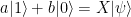
Before we explain the teleportation algorithm, let us quickly recall some definitions. Suppose that we are given a system with two qubits, say A and B. Consider the unitary operator

$U = C_{NOT} (H \otimes I)$

i.e. the operator that applies a Hadamard operator to qubit A and then a CNOT gate with control qubit A and target qubit B. Let us calculate the action of this operator on the basis state $|0 \rangle |0 \rangle$ .

$U |0 \rangle |0 \rangle = \frac{1}{\sqrt{2}} C_{NOT} (|0 \rangle |0 \rangle + |1 \rangle |0 \rangle) = \frac{1}{\sqrt{2}} (|00 \rangle + |11 \rangle)$

It is not difficult to show that this state cannot be written as a product – it is an entangled state. Traditionally, this state is called a Bell state.

Now the operator U is unitary, and it therefore maps a Hilbert space basis to a Hilbert space basis. We can therefore obtain a basis of our two-qubit Hilbert space that consists of entangled states by applying the transformation U to the elements of the computational basis. The resulting states are easily calculated and are as follows (we use the notation from [1]).

Computational basis vector	Bell basis vector
$\|00 \rangle$	$\|\beta_{00} \rangle = \frac{1}{\sqrt{2}} (\|00 \rangle + \|11 \rangle)$
$\|01 \rangle$	$\|\beta_{01} \rangle = \frac{1}{\sqrt{2}} (\|01 \rangle + \|10 \rangle)$
$\|10 \rangle$	$\|\beta_{10} \rangle = \frac{1}{\sqrt{2}} (\|00 \rangle - \|11 \rangle)$
$\|11 \rangle$	$\|\beta_{11} \rangle = \frac{1}{\sqrt{2}} (\|01 \rangle - \|10 \rangle)$

Of course we can also reverse this process and express the elements of the computational basis in terms of the Bell basis. For later reference, we note that we can write the computational basis as

$|00\rangle = \frac{1}{\sqrt{2}} (\beta_{00} + \beta_{10})$
$|01\rangle = \frac{1}{\sqrt{2}} (\beta_{01} + \beta_{11})$
$|10\rangle = \frac{1}{\sqrt{2}} (\beta_{01} - \beta_{11})$
$|11\rangle = \frac{1}{\sqrt{2}} (\beta_{00} - \beta_{10})$

Quantum teleportation

Let us now turn to the real topic of this post – quantum teleportation. Suppose that Alice is in possession of a qubit that captures some quantum state $|\psi \rangle = a |0 \rangle + b|1 \rangle$ , stored in some sort of quantum device, which could be a superconducting qubit, a trapped ion, a polarized photon or any other physical implementation of a qubit. Bob is operating a similar device. The task is to create a quantum state in Bob’s device which is identical to the state stored in Alice device.

To be able to do this, Alice and Bob will need some communication channel. Let us suppose that there is a classical channel that Alice can use to transmit a finite number of bits to Bob. Is that sufficient to transmit the state of the qubit?

Obviously, the answer is no. Alice will not be able to measure both coefficients a and b, and even if she would find a way to do this, she would be faced with the challenge of transmitting two complex numbers with arbitrary precision using a finite string of bits.

At the other extreme, if Alice and Bob were able to fully entangle their quantum devices, they would probably be able to transmit the state. They could for instance implement a swap gate to move the state from Alice device onto Bob’s device.

So if Alice and Bob are able to perform arbitrary entangled quantum operations on the combined system consisting of Alice qubit and Bob’s qubit, a transmission is possible. But what happens if the devices are separated? It turns out that a transmission is still possible based on the classical channel provided that Alice and Bob had a chance to prepare a common state before Alice prepares $|\psi \rangle$ . In fact, this common state does not depend at all on $|\psi \rangle$ , and at no point during the process, any knowledge of the state $|\psi \rangle$ is needed.

The mechanism first described in [2] works as follows. We need three qubits that we denote by A, B and C. The qubit C contains the unknown state $|\psi \rangle_C$ (we use the lower index to denote the qubit in which the state lives). We also assume that Alice is able to perform arbitrary measurements and operations on A and C, and that B similarly controls qubit B.

The first step in the algorithm is to prepare an entangled state

$|\beta_{00}^{AB} \rangle = \frac{1}{\sqrt{2}} \big[ |0\rangle _A |0 \rangle _B+ |1\rangle_A |1 \rangle_B) \big]$

Here the upper index at $\beta$ indicates the two qubits in which the Bell state vector lives. This is the common state mentioned above, and it can obviously be prepared upfront, without having the state $|\psi \rangle_C$ . Bob and Alice could even prepare an entire repository of such states, ready for being used when the actual transmission should take place.

Now let us look at the state of the combined system consisting of all three qubits.

$|\beta_{00}^{AB} \rangle |\psi\rangle_C = \frac{1}{\sqrt{2}} \big[ a |000 \rangle + a |110 \rangle + b |001\rangle + b |111 \rangle \big]$

For a reason that will become clear in a second, we will now adapt the tensor product order and choose the new order A-C-B. Then our state is (simply swap the last two qubits)

$\frac{1}{\sqrt{2}} \big[ a |000 \rangle + a |101 \rangle + b |010\rangle + b |111 \rangle \big]$

Now instead of using the computational basis for our three-qubit system, we could as well use the basis that is given by the Bell basis of the qubits A and C and the computational basis of B, i.e. $|\beta^{AC}_{ij} \rangle |k\rangle$ . Using the table above, we can express our state in this basis. This will give us four terms that contain a and four terms that contain b. The terms that contain a are

$\frac{a}{2} \big[ |\beta^{AC}_{00}\rangle |0 \rangle + |\beta^{AC}_{10}\rangle |0 \rangle + |\beta^{AC}_{01}\rangle |1 \rangle - |\beta^{AC}_{11} \rangle |1 \rangle \big]$

and the terms that contain b are

$\frac{b}{2} \big[ |\beta^{AC}_{01}\rangle |0 \rangle + |\beta^{AC}_{11}\rangle |0 \rangle + |\beta^{AC}_{00}\rangle |1 \rangle - |\beta^{AC}_{10} \rangle |1 \rangle \big]$

So far we have not done anything to our state, we have simply re-written the state as an expansion into a different basis. Now Alice conducts a measurement – but she measures A and C in the Bell basis. This will project the state onto one of the basis vectors $|\beta_{ij}^{AC}\rangle$ . Thus there are four different possible outcomes of this measurement, which we can read off from the expansion in terms of the Bell basis above.

Measurement	State of qubit B
$\beta_{00}$	$a\|0\rangle + b\|1\rangle = \|\psi \rangle$
$\beta_{01}$	$a\|1\rangle + b\|0\rangle = X\|\psi \rangle$
$\beta_{10}$	$a\|0\rangle - b\|1\rangle = Z\|\psi \rangle$
$\beta_{11}$	$b\|0\rangle - a\|1\rangle = -XZ\|\psi \rangle$

Now Alice sends the outcome of the measurement to Bob using the classical channel. The table above shows that the state in Bob’s qubit B is now the result of a unitary transformation which depends only on the measurement outcome. Thus if Bob receives the measurement outcomes (two bits), he can do a lookup on the table above and apply the inverse transformation on his qubit. If, for instance, he receives the measurement outcome 01, he can apply a Pauli X gate to his qubit and then knows that the state in this qubit will be identical to the original state $|\psi \rangle$ . The teleportation process is complete.

Implementing teleportation as a circuit

Let us now build a circuit that models the teleportation procedure. The first part that we need is a circuit that creates a Bell state (or, more generally, transforms the elements of the computational basis into the Bell basis). This is achieved by the circuit below (which again uses the Qiskit convention that the most significant qubit q₁ is the leftmost one in the tensor product).

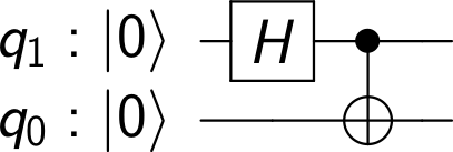
It is obvious how this circuit can be reversed – as both individual gates used are there own inverse, we simply need to reverse their order to obtain a circuit that maps the Bell basis to the computational basis.

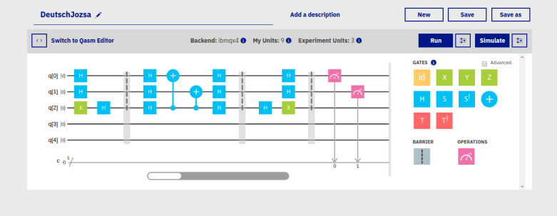
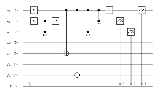
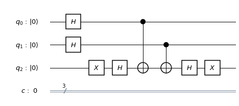
Let us now see how the overall teleportation circuit looks like. Here is the circuit (drawn with Qiskit).

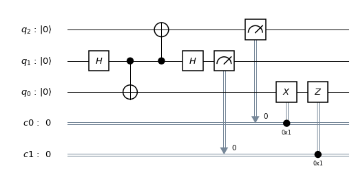
Let us see how this relates to the above description. First, the role of the qubits is, from the top to the bottom

C = q[2]
A = q[1]
B = q[0]

The first two gates (the Hadamard and the CNOT gate) act on qubits A and B and create the Bell basis vector $\beta_{00}$ from the initial state. This state is the shared entangled state that Alice and Bob prepare upfront.

The next section of the circuit operates on the qubits A and C and realizes the measurement in the Bell basis. We first use a combination of another CNOT gate and another Hadamard gate to map the Bell basis to the computational basis and then perform a measurement – these steps are equivalent to doing a measurement in the Bell basis directly.

Finally, we have a controlled X gate and a controlled Z gate. As described above, these gates apply the conditional corrections to Bob’s state in qubit B that depend on the outcome of the measurement. As a result, the state of qubit B will be the same as the initial state of qubit C.

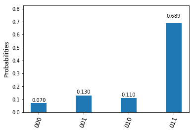
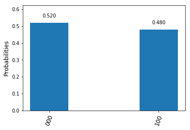
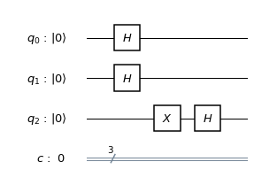
How can we test this circuit? One approach could be to add a pre-processing part and a post-processing part to our teleportation circuit. The pre-processing gate acts with one or more gates on qubit C to put this qubit into a defined state. We then apply the teleportation circuit. Finally, we apply a post-processing circuit, namely the inverse sequence of gates to the “target” of the teleportation, i.e. to qubit B. If the teleportation works, the pre- and post-steps act on the same logical state and therefore cancel each other. Thus the final result in qubit B will be the initial state of qubit C, i.e. $|0 \rangle$ . Therefore, a measurement of this qubit will always yield zero. Thus our final test circuit looks as follows.

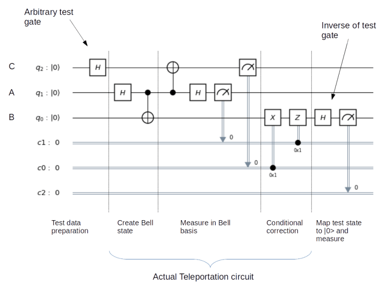
When we run this on a simulator, the result will be as expected – the value in the classical register c2 after the measurement will always be zero. I have not been able to test this on real hardware as the IBM device does not (yet?) support classical conditional gates, but the result is predictable – we would probably get the same output with some noise. If you want to play with the circuits yourself, you can, as always, find the code in my GitHub repository.

So this is quantum teleportation – not quite as mysterious as the name suggests. In particular, we do not magically teleport particles and actual matter, but simply quantum information, based on a clever split of the information contained in an unknown state into a classical part, transmitted in two classical bit, and a quantum part that we can prepare upfront. We also do not violate special relativity – to complete the process, we depend on the measurement outcomes that are transmitted via a classical channel and therefore not faster than the speed of light. It is also important to note that quantum teleportation does also not violate the “no-cloning”-principle – the measurements let the original state collapse and therefore we do not end up with two copies of the same state.

Quantum teleportation has already been demonstrated in reality several times. The first experimental verification was published in [3] in 1997. Since then, the distance between the involved parties “Alice” and “Bob” has been gradually increased. In 2017, a chinese team reported a teleportation of a single qubit between a ground observatory to a low-Earth-orbit satellite (see [4]).

The term quantum teleportation is also used in the context of quantum error correction for a circuit that uses a measurement on an entangled state to bring one of the involved qubits into a specific state. When using a surface code, for instance, this technique – also called gate teleportation – is used to implement the T gate on the level of logical qubits. We refer to [5] for a more detailed discussion of this pattern.

References

1. M. Nielsen, I. Chuang, Quantum Computation and Quantum Information, Cambridge University Press, Cambridge 2010
2. C.H. Bennett, G. Brassard, C. Crepeau, R. Jozsa, A Peres, W.K. Wootter, Teleporting an Unknown Quantum State via Dual Classical and EPR Channels, Phys. Rev. Lett. 70, March 1993
3. D. Bouwmeester, Jian-Wei Pan, K. Mattle, M. Eibl, H. Weinfurter, A. Zeilinger, Experimental quantum teleportation, Nature Vol. 390, Dec. 1997
4. Ji-Gang Ren et. al., Ground-to-satellite quantum teleportation, Nature Vol. 549, September 2017
5. D. Gottesman, I. L. Chuang, Quantum Teleportation is a Universal Computational Primitive, arXiv:quant-ph/9908010

Factoring integers on a quantum computer with Qiskit

After all the work done in the previous posts, we are now ready to actually implement Shor’s factoring algorithm on a real quantum computer, using once more IBMs Q Experience and the Qiskit framework.

First, recall that Shor’s algorithm is designed to factor an integer M, with the restriction that M is supposed to be odd and not a prime power. Thus the smallest meaningful value of M is M=15. Of course this is a toy example, but we will see that even this toy example can be challenging on the available hardware. Actually, 15 is also the number that was factored in the first implementation of Shor’s algorithm on a real quantum computer which used an NMR based device and was done in 2001 – see [1].

The quantum part of the algorithm is designed to find the period r of a chosen number a modulo M. There are several choices of a that are possible, the only condition we need is that a and M are co-prime. In this post, we follow the choice in [1] and use a = 11 and a = 7. As in [1] (and all other similar papers I am aware of, see also the discussion in this paper by Smolin, Smith which later appeared in Nature) we will also rely on prior knowledge of the result to build up our circuits, so we are actually cheating – this is not really an application of Shor’s algorithm, but merely a confirmation of a known factoring.

Of course, it is easy to compute the period directly in our case. The period of a = 11 is two, and the period of a = 7 is four. A smaller period means a simpler circuit, and therefore we start with the case a = 11. Let us see whether we can confirm the period.

The easy case – a = 11

For our tests, we will use the description of Shor’s algorithm in terms of the quantum phase estimation procedure. Thus we have a primary register that we initialize in the state $|1\rangle$ and to which we apply a sequence of controlled multiplications by powers of a, and a working register, in which we do a quantum Fourier transform in the second step. The primary register needs to hold M=15, so we need four qubits there. For the working register, we use three qubits, which is the smallest possible choice, to keep the number of gates small.

The first step of our algorithm is controlled multiplication by a. However, this is greatly simplified by the fact that we apply this to exactly one state that we know upfront – the initial state $1 \rangle$ . Thus we only need to implement a unitary transformation which conditionally maps the state $|1 \rangle$ to the state $|a = 11 \rangle$ . In binary notation, eleven is 1011, and we therefore simply need to conditionally flip qubits 3 and 1. We also need a Pauli X gate in the primary register to build the initial state $|1 \rangle$ from the fiducial state $|0\rangle$ and Hadamard gates in the working register to create the initial superposition. Thus the first part of our circuit looks as follows.

What about higher powers of a? This is easy – we know that a² is equal to one modulo M, and therefore the multiplication by a² modulo M is simply the identity transformation. The same is true for all even powers and so we are already done with the first part of our circuit – this is why we call the case a = 11 the easy case. The only thing that is left is to add the quantum Fourier transformation and a measurement to the working register. This gives us the following circuit (which can obviously be simplified, more on this later).

Now we can run this on a simulator. Before we do this, let us try to understand what we expect. We know that after measuring the working register, the value that we obtain is a multiple of 2³ / r = 8 / 2 = 4. Thus we expect to see peaks at 0 and four (binary 100). And this is actually what we get – the following histogram shows the output of an execution on the local QASM simulator integrated into Qiskit.

This is nice, our circuit seems to work correctly. So let us proceed and try this on real hardware. Before we do so, however, let us simplify our circuit a bit to reduce the number of gates needed and thus the noise level. First, we skip the final swap gates in the QFT circuit – this will change our expected output from 100 to 001, but we can keep track of this manually when setting up the measurement. Next, we have two Hadamard gates on w[2] that cancel and that we can therefore remove. And the Pauli X gate on p[0] is never really used and can be dropped. After these changes, we obtain the following circuit.

We can run this on the IBMQ hardware. As we require seven qubits in total, we need to do this on the 14 qubit model ibmq_16_melbourne. Here are the results of a test run, again as a histogram.

We see the expected peaks at 000 and 100, but also see some significant noise that is of course not present in the simulation. However, the probabilities to measure one of the theoretically expected values is still roughly twice as high as the probability of any of the other values.

The hard case – a = 7

Having mastered the case a = 11, let us now turn to the case a = 7. The only change that we need to make is the circuit acting on the primary register. In the first part of the circuit, we can again make use of the fact that we only have to deal with one possible input, namely the initial state $|1 \rangle$ . The conditional multiplication by a maps this to $|7\rangle$ , and we can again implement this by two conditional bit flips, i.e. two CNOT gates.

The second part, the conditional multiplication by a² = 4 modulo M, requires a bit more gates. On a bit level, multiplication by four is a bit shift by two bits to the left. We can realize this as a sequence of two conditional swap gates, swapping the bits zero and two and the bits one and three. A conditional swap gate can be implemented by three CNOT gates, or, in QASM syntax,

gate cswap a,b,c
{
  cx c,b;
  ccx a,b,c;
  cx c,b;
}

We can also make a few simplifications by replacing CNOT gates with fixed values of the control qubit by either an inversion or the identity. We arrive at the following circuit.

This is already considerably more complex than for the case a = 11. When we add the QFT circuit and the measurements, we end up with the following circuit.

Now the period is four. Thus we expect peaks at all multiples of two, i.e. at all even values. And this is actually what we get when we run this on a simulator.

Now let us again see how we can optimize this circuit before trying it on real hardware. Again, there are a few additional simplifications that we can make to reduce the noise level. On w[2], we have a double Hadamard gate that we can remove. We can again dispose of the final swap gates and move the swap operation into the measurement. The last CNOT between p[1] and p[3] can be dropped as it does not affect the outcome. The same is true for the last CNOT between p[0] and p[2]. Thus we finally arrive at the following circuit.

And here is the result of running this on the 16 qubit IBM device.

Surprisingly, the noise level is not significantly worse than for the version with a = 11, even though we have a few more gates. We can clearly see that the probabilities to measure even values are significantly higher than the probabilities to measure odd values, corresponding to the period four.

So what did we learn from all this? First, our example was of course a toy model – we did code the circuit based on knowledge on the period and hard-coded the value of a. However, our example demonstrates the basic techniques to build circuits for the more general case. In real application, we could, given a number M, first determine a suitable value for a. The conditional multiplication by a is then acting as a permutation on the computational basis and can therefore be implemented by a sequence of (conditional) swap gates. The same is true for higher powers of a. So in theory, we have all the ingredients that we need to implement more general versions of the algorithm.

In practice, however, we will quickly reach a point where the number of gates exceeds the limit that we can reasonable implement given the current level of noise. So real applications of the algorithm in number ranges that are not tractable for classical digital computers will require advanced error correction mechanisms and significantly reduced noise levels. Still, it is nice (and fun) to see a toy version of the famous algorithm in action on a real device.

If you want to run the examples yourself, you can use my notebooks for the case a=11 and a=7.

References

1. L. Vandersypen, M. Steffen, G. Breyta, C. Yannoni, M. Sherwood, I. Chuang, Experimental realization of Shor’s quantum factoring algorithm using nuclear magnetic resonance, Nature Vol. 414, (December 2001)
2. P. Shor, Polynomial-Time Algorithms for Prime Factorization and Discrete Logarithms on a Quantum Computer, SIAM J.Sci.Statist.Comput. Vol. 26 Issue 5 (1997), pp 1484–1509, available as arXiv:quant-ph/9508027v2
3. R. Cleve, A. Ekert, C. Macchiavello, M. Mosca, Quantum Algorithms revisited, arXiv:9708016
4. A. Kitaev, Quantum measurements and the Abelian Stabilizer Problem, arXiv:quant-ph/9511026
5. J. Smolin, G. Smith, A. Vargo, Pretending to factor large numbers on a quantum computer, arXiv:1301.7007 [quant-ph]

Implementing the quantum Fourier transform with Qiskit

The quantum Fourier transform is a key building block of many quantum algorithms, from Shor’s factoring algorithm over matrix inversion to quantum phase estimation and simulations. Time to see how this can be implemented with Qiskit.

Recall that the quantum Fourier transform (or, depending on conventions, its inverse) is given by

$|x \rangle \mapsto \frac{1}{\sqrt{2^n}} \sum_s \eta^{xs} |s \rangle$

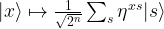
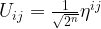
where $\eta$ is an 2ⁿ-th root of unity with n being the number of qubits in the register, i.e.

$\eta = \exp \frac{2\pi i}{2^n}$

How can we effectively create this state with a quantum circuit? They key to this is the observation (see the references below) that the result of the quantum Fourier transform can be written as a product state, namely as

$\sum_s \eta^{xs} |s \rangle = (|0\rangle + \eta^{2^{n-1} x}|1\rangle)(|0 \rangle + \eta^{2^{n-2}x}|1 \rangle) \cdots (|0 \rangle + \eta^x|1 \rangle)$

which you can easily verify by multiplying out the product and collecting terms.

Here we use the tensor product order that is prescribed by OpenQASM, i.e. the most significant bit is q[n-1]. This bit is therefore given by

$|0 \rangle + \eta^{2^{n-1}x} |1 \rangle$

Let us analyse this expression further. For that purpose, we decompose x into its representation as a binary number, i.e. we write

$x = \sum_{i=0}^{n-1} 2^i x_i$

with x_i being the binary digits of x. If we now multiply this by 2^n-1, we will get $2^{n-1} x_0$ plus a multiple of 2ⁿ. As $\eta$ is a root of unity, this multiple cancels out and we obtain that

$\eta^{2^{n-1}x} = \eta^{2^{n-1}x_0} = e^{\pi i x_0} = (-1)^{x_0}$

Thus, we can write the most significant qubit of the Fourier transform as

$|0 \rangle + (-1)^{x_0} |1 \rangle$

which is nothing but

$H |x_0\rangle$

Thus we obtain the most significant qubit of the quantum Fourier transform by simply applying a Hadamard gate to the least significant qubit of the input.

This is nice and simple, but what about the next qubit, i.e. qubit n-2? From the decomposition above, we can see that this is simply

$|0 \rangle + \eta^{2^{n-2}x} |1 \rangle$

Using exactly the same arguments as for the most significant qubit, we easily find that this is

$|0 \rangle + \eta^{2^{n-2}x_0} H |x_1 \rangle$

Thus we obtain this qubit from qubit 1 by first applying a Hadamard gate and then a conditional phase gate, i.e. a conditional rotation around the z-axis, conditioned on the value of x₀. In general, qubit n-j is

$|0 \rangle + \prod_{i < j - 1} \eta^{2^{n-j+i}x_i} H |x_{j-1}\rangle$

which is a Hadamard gate followed by a sequence of conditional rotations around the z-axis, conditioned on the qubits with lower significance.

So we find that each qubit of the Fourier transform is obtained by applying a Hadamard followed by a sequence of conditional rotations. However, the order of the qubits in the output is reversed, i.e. qubit n-j is obtained by letting gates act on qubit j. Therefore, at the end of the circuit, we need to revert the order of the qubits.

In OpenQASM and Qiskit, a conditional rotation around the z-axis is called CU1, and there are swap gates that we can use to implement the final reversing of the qubits. Thus, we can use the following code to build a quantum Fourier transformation circuit acting on n qubits.

def nBitQFT(q,c,n):
    circuit = QuantumCircuit(q,c)
    #
    # We start with the most significant bit
    #
    for k in range(n):
        j = n - k
        # Add the Hadamard to qubit j-1
        circuit.h(q[j-1])
        #
        # there is one conditional rotation for
        # each qubit with lower significance
        for i in reversed(range(j-1)):
            circuit.cu1(2*np.pi/2**(j-i),q[i], q[j-1])
    #
    # Finally we need to swap qubits
    #
    for i in range(n//2):
        circuit.swap(q[i], q[n-i-1])
    return circuit

Here is the circuit that this code produces for n=4. We can clearly see the structure – on each qubit, we first act with a Hadamard gate, followed by a sequence of conditional rotations with decreasing angle, conditioned on the less significant qubits, and finally reorder the qubits.

This is already a fairly complex circuit, and we need to find a way to test it. Let us look at the options we have. First, a quantum circuit is a unitary transformation and can be described by a matrix. In our case, it is especially easy to figure out what this matrix should be. Looking at the formula for the quantum Fourier transform, we find that the matrix describing this transformation with respect to the computational basis has the elements

$U_{ij} = \frac{1}{\sqrt{2^n}} \eta^{ij}$

The Qiskit frameworks comes with a simulator called the unitary_simulator that accepts a quantum circuit as input and returns the matrix describing that circuit. Thus, one possible test approach could be to build the circuit, run the unitary simulator on it, and to compare the resulting unitary matrix with the expected result given by the formula above. In Python, the expected result is produced by the following code

def qftMatrix(n):
    qft = np.zeros([2**n,2**n], dtype=complex)
    for i in range(2**n):
        for j in range(2**n):
            qft[i,j] = np.exp(i*j*2*1j*np.pi/(2**n))
    return 1/np.sqrt(2**n)*qft

and the test can be done using the following function

def testCircuit(n):
    q = QuantumRegister(n,"x")
    c = ClassicalRegister(n,"c")
    circuit = nBitQFT(q,c,n)

    backend = Aer.get_backend('unitary_simulator')
    job = execute(circuit, backend)
    actual = job.result().get_unitary()
    expected = qftMatrix(n)
    delta = actual - expected
    print("Deviation: ", round(np.linalg.norm(delta),10))
    return circuit

The outcome is reassuring – we find that the matrices are the same within the usual floating point rounding differences.

After passing this test, a next reasonable validation step could be to run the algorithm on a specific input. We know that the QFT will map the state $|0 \rangle$ into an equal superposition of all elements of the computational basis. Conversely, we therefore expect that if we start with such a superposition, the QFT will map the superposition onto $|0\rangle$ , at least up to a phase.

Let us try this out. Our test circuit will consist of a layer of Hadamard gates to create the equal superposition, followed by the QFT circuit, followed by a measurement. The resulting circuit for n=4 is displayed below.

It we run this circuit on the QASM simulator embedded into Qiskit, the result is as expected – for 1024 shots, we get 1024 times the output ‘0000’. So our circuit works – at least theoretically. But what about real hardware?

Let us compile and run the circuit targeting the IBM Q Experience 14 qubit device. If we dump the QASM code after compilation, we see that the overall circuit will have roughly 140 gates. This is already significant, and we expect to see some noise. To see how bad it is, I have conducted several test runs and plotted the results as a histogramm (if you want to play with this yourself, you will find the notebook on Github). Here is the output of a run with n=4.

We still see a clear peak at the expected result, but also see that the noise level is close to making the result unusable – if we did not know the result upfront, we would probably not dare to postulate anything from this output. With only three qubits, the situation becomes slightly better but is still far from being satisfactory.

Of course we could now start to optimize the circuit – remove cancelling Hadamard gates, remove the final swap gates, reorder qubits to take the coupling map into account and so on – but it becomes clear that with the current noise level, we are quickly reaching a point where even comparatively simple circuit will inflict a level of noise that is at best difficult to handle. Hopefully, this is what you expected after reading my posts on quantum error correction, but I found it instructive to see noise in action in this example.

References

1. M. Nielsen, I. Chuang, Quantum Computation and Quantum Information, Cambridge University Press 2010
2. R. Cleve, A. Ekert, C. Macchiavello, M. Mosca, Quantum Algorithms revisited, arXiv:9708016

Running the Deutsch-Jozsa algorithm on IBMs Q experience

In one of the previous posts, we have looked at the basics of the Qiskit package that allows us to create and run quantum algorithms in Python. In this post, we will apply this to model and execute a real quantum algorithm – the Deutsch-Jozsa algorithm.

Recall that the Deutsch-Jozsa algorithm is designed to solve the following problem. We are given a boolean function f

$f \colon \{0,1\}^n \rightarrow \{0,1\}$

in n variables. We know that the function is either constant or it is balanced (i.e. the number of times it is zero is equal to the number of times it is equal to 1). The task is to determine which of the to properties – balanced or constant – the function f has.

The first choice that we need to make is of course a suitable function f. To keep things simple, we will use a function with two variables. Maybe the most straightforward example for a balanced function in two variables is the classical XOR function.

$f(x_0, x_1) = x_0 \oplus x_1$

Thus our first task is to develop a quantum equivalent of this function, i.e. a reversible version of f.

Recall that in general, given a boolean function f, we can define a unitary transformation U_f by the following rule

$U_f(|x \rangle |y \rangle) = |x \rangle |y \oplus f(x) \rangle$

Thus U_f flips the target qubit y if f(x) is one and leaves it unchanged otherwise. In our case, combining this with the definition of the XOR function implies that we are looking for a circuit acting on three qubits – two input qubits and one target qubit – that flips the target qubit if and only if the two input qubits are not equal. From this textual description, it is obvious that this can be constructed using a sequence of two CNOT gates.

Let us now go through the individual steps of the Deutsch-Jozsa algorithm, using the optimized version published 1997 in this paper by R. Cleve, A. Ekert, C. Macchiavello and M. Mosca (this version is also described in one of my earlier posts but is does not hurt to recap some of that). The first step of the algorithm is to prepare a superposition state

$|\psi_0 \rangle = \frac{1}{2} \sum_x |x \rangle$

This is accomplished by applying a Hadamard gate to each of the two qubits that make up our primary register in which the variable x lives. We then add an ancilla qubit that is in the state $H|1 \rangle$ , so that our state is now

$\frac{1}{2} \sum_x |x \rangle \otimes H |1 \rangle = \frac{1}{2\sqrt{2}} \sum_x |x , 0 \rangle - |x, 1 \rangle$

So far our circuit looks as follows.

Next we apply the oracle U_f to our state. According to the definition of the oracle, we have

$U_f |x, 0 \rangle = |x\rangle |f(x) \rangle$

and

$U_f |x, 1 \rangle = |x\rangle |f(x) \oplus 1\rangle$

Therefore we find that

From this formula, we can read off how U_f acts depending on the value of f(x). If f(x) is 0, the right hand side is equal to the left hand side and U_f acts trivially. If, however, f(x) is one, the right hand side is simply minus the left hand side, and U_f acts as multiplication by -1. Combining this with our previous formula, we obtain

$U_f \colon: \frac{1}{2} \sum_x |x \rangle \otimes H |1 \rangle \mapsto \frac{1}{2} \sum_x (-1)^{f(x)}|x \rangle \otimes H |1 \rangle$

Next, we apply again the Hadamard operator followed by the Pauli X gate to the third qubit (the ancilla), i.e. we uncompute the ancilla qubit. From the expression above, we can read off directly that the result left in the first two qubits will be

$|\psi \rangle = \frac{1}{2} \sum_x (-1)^{f(x)}|x \rangle$

This is the vector that we will have in the first two qubits of our quantum register when we have processed the following circuit.

Let us now calculate the overlap, i.e. the scalar product, between this vector and the initial superposition $|\psi_0 \rangle$ . Clearly,

$\langle \psi_0 |\psi \rangle = \frac{1}{4} \sum_x (-1)^{f(x)}$

We find that this overlap is zero if and only if the function f is balanced. But how can we measure this scalar product? To see this, recall that the initial state $|\psi_0 \rangle$ is the result of applying the tensor product H² of the two Hadamard operators to the first two qubits in the fiducial state. Thus we can write our scalar product as

$\langle \psi_0 |\psi \rangle = \langle 0 | H^2 |\psi \rangle = \langle 0 | H^2 \psi \rangle$

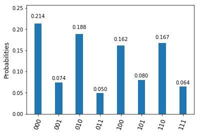
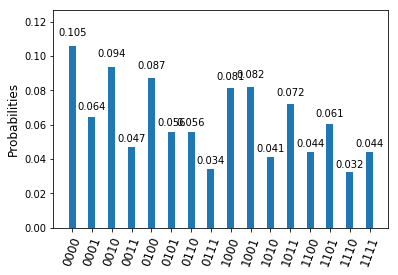
In other words, we can determine the scalar product by again applying a Hadamard operator to each of the first two qubits and measuring the overlap of the resulting state with the basis state $|00 \rangle$ which is the same thing as the probability to measure $|00 \rangle$ when we perform a measurement in the computational basis. Thus we finally obtain the following circuit

and the function f is balanced if and only if the probability to measure $|00 \rangle$ is zero.

Let us now turn this into Python code using Qiskit. I found it useful to create subroutines that act on a given circuit and build parts of the circuit which can then be tested independently from each other on a simulator before combining them. Here is the code to create the oracle for our balanced function f.

def createOracleBalanced(q,c):
    circuit = QuantumCircuit(q,c)
    circuit.cx(q[0], q[2])
    circuit.cx(q[1], q[2])
    circuit.barrier(q)
    return circuit

Similarly, we can write routines that create the initial state and join the ancilla qubit.

def createInitialState(circuit):
    circuit.h(q[0])
    circuit.h(q[1])
    circuit.barrier(q)

def addAncilla(circuit):
    circuit.x(q[2])
    circuit.h(q[2])
    circuit.barrier(q)

Finally, we need to be able to uncompute the ancilla and to add the final measurements.

def uncomputeAncilla(circuit):
    circuit.h(q[2])
    circuit.x(q[2])
    circuit.barrier(q)

def addMeasurement(circuit):
    circuit.h(q[0])
    circuit.h(q[1])
    circuit.barrier(q)
    circuit.measure(q[0], c[0])
    circuit.measure(q[1], c[1])
    circuit.barrier(q)

A word on barriers. In this example code, we have added barriers after each part of the circuit. Barriers are an element of the OpenQASM specification and instruct the compiler not to combine gates placed on different sides of a barrier during optimization. In Qiskit, barriers have the additional benefit of structuring the visualization of a circuit, and this is the main reason I have included them here. In an optimized version, it would probably be safe to remove them.

After all these preparations, it is now easy to compile the full circuit. This is done by the following code snippet – note that we can apply the + operator to two circuits to tell Qiskit to concatenate the circuits.

q = QuantumRegister(3,"q")
c = ClassicalRegister(3,"c")
circuit = QuantumCircuit(q,c)
createInitialState(circuit)
addAncilla(circuit)
circuit = circuit + (createOracleBalanced(q,c))
uncomputeAncilla(circuit)
addMeasurement(circuit)

We can then compile this code for a simulator or a backend as explained in my last post on the IBM Q experience (you can also find the full source code here). The following histogramm shows the result of the final measurement after running this on the ibmqx4 5 qubit quantum computer.

We see, as in the experiments conducted before, that the theoretically expected result (confirmed by running the circuit on a simulator) is blurred by noise – we get the value 00 in a few instances, even though the function is balanced. Even though the outcome can still be derived with a reasonable likelihood, we start to get a feeling for the issues that we might have with noise for more complex functions and circuits.

It is instructive to extract the compiled QASM from the resulting qobj and load that code into the IBM Q Experience composer. After a few beautifications, the resulting code (which you can get here) is displayed as follows in the composer.

If we compare this to the original circuit, we see that the compiler has in fact rearranged the CNOT gates that make up our oracle. The reason is that the IBMQX4 device can only realize specific CNOT gates. It can, for instance, implement a CNOT gate with q[1] as control as q[0] as target, but not vice versa. Therefore the compiler has added Hadamard gates to swap control and target qubit. We also see that the compiler has respected the barriers and not cancelled some of the double Hadamard gates. If we remove the barriers and remove all Hadamard gates that clearly cancel each other, we finally obtain a greatly simplified version of the circuit which looks as follows.

Of course this simplification hinges on the special choice of the function f. Nevertheless, it is useful – fewer gates mean fewer errors. If we compare the error rates of the optimized circuit with the new circuit, we find that while the original version had an error (i.e. an unexpected amplitude of $|00 \rangle$ ) of roughly 10%, a run with the optimized circuit showed an error of only 5,5%.

This completes our post. The next algorithm that we will implement is Shor’s algorithm and the quantum Fourier transform.

Computational basis vector	Bell basis vector
$\|00 \rangle$	$\|\beta_{00} \rangle = \frac{1}{\sqrt{2}} (\|00 \rangle + \|11 \rangle)$
$\|01 \rangle$	$\|\beta_{01} \rangle = \frac{1}{\sqrt{2}} (\|01 \rangle + \|10 \rangle)$
$\|10 \rangle$	$\|\beta_{10} \rangle = \frac{1}{\sqrt{2}} (\|00 \rangle - \|11 \rangle)$
$\|11 \rangle$	$\|\beta_{11} \rangle = \frac{1}{\sqrt{2}} (\|01 \rangle - \|10 \rangle)$