
In the previous post, we have looked at the basic ideas behind quantum error correction, namely the encoding of logical states so that we are able to detect and correct errors like bit flip and phase flip errors. Unfortunately, this is not yet good enough to implement quantum computing in a fault-tolerant way.
What is still missing? First, we have only discussed errors that impact saved quantum states, i.e. random bit flips or phase flips that invalidate a given state stored in a quantum register. We have not yet, however, understood how we can protect quantum states during processing, i.e. deal with errors that do not occur on a saved qubit but that occur while we manipulate these qubits by executing quantum gates.
Second, and maybe even worse, implementing error correction involves adding additional qubits and quantum gates to our circuit. Obviously, these additional elements will again be subject to errors and require protection. So we might need an additional correction step to account for these errors. This additional step will again introduce additional errors and so forth. It is not a priori clear that we do not introduce more errors than we can correct when following this path. Fortunately, the famous threshold theorem asserts that under certain conditions, we can win this race and correct errors faster than we create them.
Error propagation and transversal quantum gates
But let us start with the first question – how can we implement quantum gates in a fault tolerant way? To illustrate the challenge, we start with a simple (though unrealistic) example. Suppose that we wanted to perform a CNOT gate on two states encoded with the three-bit code. The obvious approach – decode the two input states, apply an ordinary CNOT and encode again – does not appear to be a good choice, as uncontrolled errors might sneak in while the states are unencoded and therefore vulnerable. So let us try to implement a CNOT operation directly on the encoded states. This can be done with the following circuit.

Let us see why this circuit works. Suppose the control word is the encoded (logical) state

Then all three qubits in the control word are zero. Consequently, the three CNOT gates do nothing and the target word is not changed. If, on the other hand, the control word is

then all three qubits in the target word will be toggled, and thus the target word 

However, there is a problem with this circuit. To see this, suppose that there is a bit flip error in the first qubit of the control word. Then this error will make all three CNOT gates toggle their target state, and a logical 
Obviously, the propagation of errors can never be entirely avoided. However, what we can avoid is the uncontrolled propagation. To explain this, let us take a look at the following circuit.

This circuit also realizes a CNOT on the level of logical states. However, for this circuit, an error in one of the qubits of the block of three qubits that encode the logical control bit can only propagate into one qubit in the second block – the block of three qubits that encode the target bit. Therefore one error per input block will only propagate into one error in each output block. If we are able to fully recover from one qubit errors per block, we can detect and correct the errors even though they have propagated through the circuit (again as long as only one error occurs). Thus the trick is to somehow spread potential errors across multiple blocks so that no single block is fully corrupted. This connectivity property of a circuit is sometimes called transversality.
Transversal gates are fault-tolerant, as an error in one qubit can only propagate into one qubit of any other code block, a situation from which we can recover. For many codes, many basic gates can be implemented qubit-wise and therefore transversally on the level of logical qubits. Unfortunately, a full set of universal quantum gates cannot be constructed in such a way – typically one gate remains for which no transversal implementation can be found. Fortunately, there are other (considerably more complicated) methods available to construct fault-tolerant logical gates. In [1], Shor has described the first fully universal set of fault-tolerant logical gates for his nine qubit code. In many modern implementations, a class of codes called surface codes are used, that also allow us to implement a universal set of quantum gates in a fault tolerant way and that we will study in a later post. Similar approaches work for measurements that can have errors as well and that need to be organized in a way so that errors can be detected and corrected, and the same applies for the actual error correction circuits.
Fault tolerant quantum computation and the threshold theorem
Even if we are able to implement quantum gates in a fault tolerant way, one challenge remains. So far, we have only discussed how to protect against single qubit errors. Of course, the rationale behind this was the assumption that errors in two or more qubits are much less probable than single qubit errors. Thus, we have reduced the error probability. For real applications, our new, reduced error probability might still not be sufficient. We therefore might have to add additional error correction circuits. Now the probability of failure for a circuit is not only a function of the reliability of every single component, but also a function of the number of components. The more error correction mechanisms we add, the higher the number of components and the higher the overall fault probability. In the worst case, the increase of the fault probability by adding the additional components needed for the error correction might eat up all the benefits of the error correction and lead to an overall higher probability of failure.
To be able to better grasp the problem, let us introduce some terminology. Suppose we are given a circuit C that describes a quantum computation. We can think of the overall computation as being organized in individual time steps. At each time step, every qubit in the circuit takes part in a basic set of possible operations (or, to mention a different term that is sometimes used, locations). This can be a gate, the preparation of a qubit in a initial state, a measurement or a “wait step”, i.e. the identity operation leaving the involved qubits unchanged. At each time step, a qubit is involved in exactly one of these operations.
Given such a circuit, we can now try to build a fault tolerant circuit performing the same computation as follows. We replace each qubit in the circuit C by a block of qubits encoding a logical qubit. Similarly, we replace each operation in C by the corresponding fault tolerant equivalent, i.e. we replace each gate by the corresponding logical gate, a measurement by a fault tolerant measurement, and a preparation by a fault tolerant state preparation. In addition, we place a (fault tolerant) error correction circuit in each block which is the output of a logical gate. The result is called a simulation of the original circuit. An example is displayed below, using (roughly) the graphical language described in [2].
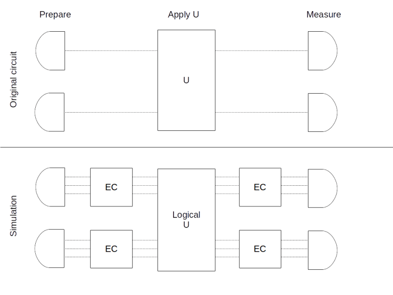
The upper part of this diagram shows an original circuit, in which we prepare two qubits in a known state, then apply the unitary transformation U and finally measure both qubits. The result of the replacement procedure described above is displayed in the lower part of the picture, using again the (unrealistic) example of a three qubit code. Here we have replaced each qubit by a corresponding block of three qubits holding the code word. The operation U has been replaced by its logical implementation, acting on the encoded states, and both after the preparation and after applying U, we add a circuit performing error correction.
Let us now study how the fault probability changes when we pass to a simulation. In general, this is a long and complicated argument, and we refer the reader to [3], [4] and [5] for the details. However, there is a simple example that can be used to illustrate some of the key ideas.
In fact, let us go back to the circuit above that we have used for a fault-tolerant implementation of the CNOT gate. To analyze the probability that this circuit fails, let us assume that the only error that can occur is a bit flip error in the target qubit of each physical CNOT gate and that this error occurs with probability p. Thus we assume that error correction, state preparation and measurement work in an idealized, error free way.
Let us now look at the different combinations of faults that can occur during a specific run of the simulation circuit, i.e. a different fault paths. A first fault path is given by a single bit flip error in one of the target qubits after executing the CNOT operation. However, this affects only one qubit and can therefore be corrected by the error correction circuit. Thus, for this fault path, the simulation works correctly.
There is, however, a different fault path, given by a fault in target qubit one and target qubit two, whereas the CNOT acting on target qubit three operates correctly. Assuming that the individual faults are statistically independent, the probability for this fault path is

This would introduce an error from which we could not recover, as our code is only able to correct errors in one qubit. But this is not yet the overall probability of failure for our new circuit, as there is a second fault path that we need to consider – we could as well have a failure in the first and the third instead of the first and second qubit. Obviously, the probability for this fault path is the same. And there is a third fault path with two errors, given by an error in the second and third target qubit. These three different fault paths, all with two errors, correspond to the

possibilities to choose two error locations out of the three target qubits. And finally, it might happen that faults occur in all three locations, an event which clearly has probability p3. Thus the overall probability to have at least two faults is

Thus the overall probability that the circuit does not operate correctly does not reduce from p – for the physical CNOT operation without error protection – to p2, but to 3 p2, where the factor 3 reflects the growth of the circuit when passing from the physical circuit to the simulation, i.e. the impact of the additional gates.
Of course this is a very simplified example, but the hard work done in the original papers in the references demonstrates that the result is true in general: if we pass from a circuit to its simulation, the change of the error rate is described by a rule of the form

where c is a constant that reflects the growth of the circuit and t is the number of errors that the code that we use can still correct. Obviously, this does not help unless the right hand side is smaller than the left hand side, i.e. unless p is smaller than a threshold given by

If this is true, we can even iterate the procedure, and reduce the error rate below every prescribed level by adding additional layers of simulation. Thus given physical operations with error rate less than pcrit, we can implement each quantum circuit in a fault-tolerant way with arbitrary reliability.
Unfortunately, the exact value of the threshold is not known. The initial estimate provided in [3] was in the range of 10-6. Later, this was improved by several authors, and is mostly assumed to be in the range between 10-4 and 10-2 (see [6] for an overview of some results in this direction).
As c is in the order of pcrit-t, this implies that we need as many as a few hundred to a few thousand physical gates and qubits to simulate one logical qubit. Note that in general, the overhead depends on the desired accuracy and the level of simulations needed as well as on the factors entering the constant c, i.e. the encoding, the architecture of the logical gates, as well as how close the actual physical error rate is to the threshold. Improving the threshold and thereby reducing the overhead remains one of the most active areas of current research in quantum computing and is essential for paving the road towards a large-scale fully fault tolerant universal quantum computer.
At the time of writing, a class of codes known as surface codes appear to be good candidates for the implementation of fault-tolerant quantum computers, not only because these codes have good error correction properties, but also because they are well adapted to the geometry of the actual quantum computer. In the next few posts, we will work towards understanding surface codes and other topological codes, starting with the formalism of stabilizer codes that will be the focus of the next post.
1. P. Shor, Scheme for reducing decoherence in quantum computer memory, Phys. Rev. A Vol. 52 (1995) Issue 4, pp. 2493–2496
2. D. Gottesman, An Introduction to Quantum Error Correction and Fault-Tolerant Quantum Computation, arXiv:0904.2557v1
3. D. Arahonov, M. Ben-Or, Fault Tolerant Quantum Computation with Constant Error, arXiv:quant-ph/9611025
4. E. Knill, R. Laflamme, W.H. Zurek, Threshold accuracy for quantum computation, arXiv:quant-ph/9610011,
5. P. Aliferis, D. Gottesman, J. Preskill, Quantum accuracy threshold for concatenated distance-3 codes, arXiv:quant-ph/0504218v3
6. S. J. Devitt, W. J. Munro, K. Nemoto, Quantum Error Correction for Beginners, arXiv:0905.2794v4

1 Comment