OpenStack Neutron – deep dive into flat and VLAN networks

Having installed Neutron in my last post, we will now analyze flat networks and VLAN networks in detail and see how Neutron actually realizes virtual Ethernet networks. This will also provide the basic understanding that we need for more complex network types in future posts.

Setup

To follow this post, I recommend to repeat the setup from the previous post, so that we have two virtual machines running which are connected by a flat virtual network. Instead of going through the setup again manually, you can also use the Ansible scripts for Lab5 and combine them with the demo playbook from Lab6.

git clone https://github.com/christianb93/openstack-labs
cd openstack-labs/Lab5
vagrant up
ansible-playbook -i hosts.ini site.yaml
ansible-playbook -i hosts.ini ../Lab6/demo.yaml

This will install a demo project and a demo user, import an SSH key pair, create a flavor and a flat network and bring up two instances connected to this network, one on each compute node.

Analyzing the virtual devices

Once all instances are running, let us SSH into the first compute node and list all network interfaces present on the node.

vagrant ssh compute1
ifconfig -a

The output is long and a bit daunting. Here is the output from my setup, where I have marked the most relevant sections in red.

FlatNetworkIfconfig

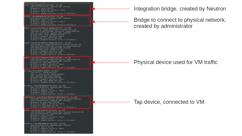
The first interface that we see at the top is the integration bridge br-int which is created automatically by Neutron (in fact, by the Neutron OVS agent). The second bridge is the bridge that we have created during the installation process and that is used to connect the integration bridge to the physical network infrastructure – in our case to the interface enp0s9 which we use for VM traffic. The name of the physical bridge is known to Neutron from our configuration file, more precisely from the mapping of logical network names (physnet in our case) to bridge devices.

The full output also contains two devices (virbr0 and virbr0-nic) that are created by the libvirt daemon but not used.

We also see a tap device, tapd5fc1881-09 in our case. This tap device is realizing the port of our demo instance. To see this, source the credentials of the demo user and run openstack port list to see all ports. You will see two ports, one corresponding to each instance. The second part of the name of the tap device matches the first part of the UUID of the corresponding port (and we can use ethtool -i to get the driver managing this interface and see that it is really a tap device).

The virtual machine is listening on the tap device and using it to provide the virtual NIC to its guest. To verify that QEMU is really listening on this tap device, you can use the following commands (run this and all following commands as root).

# Figure out the PID of QEMU
pid=$(ps --no-headers \
      -C qemu-system-x86_64 \
      | awk '{ print $1}')
# Search file descriptors in /proc/*/fdinfo 
grep "tap" /proc/$pid/fdinfo/*

This should show you that one of the file descriptors is connected to the tap device. Let us now see how this tap device is attached to the integration bridge by running ovs-vsctl show. The output should look similar to the following sample output.

4629e2ce-b4d9-40b1-a362-5a1ba7f79e12
    Manager "ptcp:6640:127.0.0.1"
        is_connected: true
    Bridge br-phys
        Controller "tcp:127.0.0.1:6633"
            is_connected: true
        fail_mode: secure
        Port phy-br-phys
            Interface phy-br-phys
                type: patch
                options: {peer=int-br-phys}
        Port "enp0s9"
            Interface "enp0s9"
        Port br-phys
            Interface br-phys
                type: internal
    Bridge br-int
        Controller "tcp:127.0.0.1:6633"
            is_connected: true
        fail_mode: secure
        Port "tapd5fc1881-09"
            tag: 1
            Interface "tapd5fc1881-09"
        Port int-br-phys
            Interface int-br-phys
                type: patch
                options: {peer=phy-br-phys}
        Port br-int
            Interface br-int
                type: internal
    ovs_version: "2.11.0"

Here we see that both OVS bridges are connected to a controller listening on port 6633, which is actually the Neutron OVS agent (the manager in the second line is the OVSDB server). The integration bridge has three ports. First, there is a port connected to the tap device, which is an access port with VLAN tag 1. This tagging is used to separate traffic on the integration bridge belonging to two different virtual networks. The VLAN ID here is called the local VLAN ID and is only valid per node. Then, there is a patch port connecting the integration bridge to the physical bridge, and there is the usual internal port.

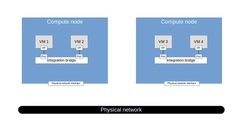
The physical bridge has also three ports – the other side of the patch port connecting it to the integration bridge, the internal port and finally the physical network interface enp0s9. Thus the following picture emerges.

FlatNetworkTopology

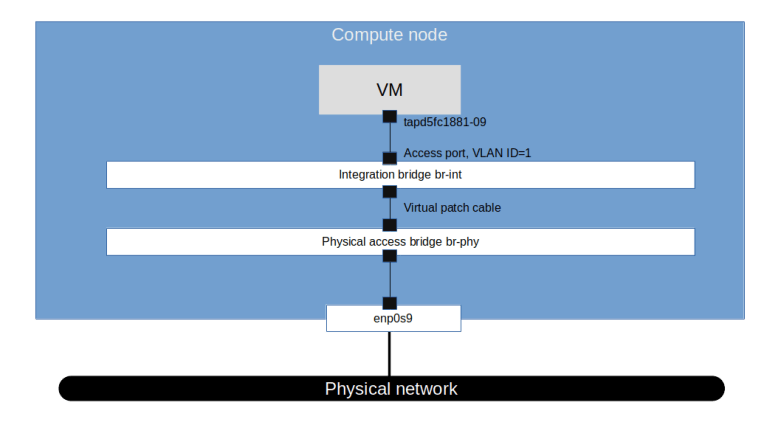
So we get a first idea of how traffic flows. When the guest sends a packet to the virtual interface in the VM, it shows up on the tap device and goes to the integration bridge. It is then forwarded to the physical bridge and from there to the physical interface. The packet travels across the physical network connecting the two compute nodes and there again hits the physical bridge, travels along the virtual patch cable to the integration bridge and finally arrives at the tap interface.

At this point, it is important that the physical network interface enp0s9 is in promiscuous mode. In fact, it needs to pick up traffic directed to the MAC address of the virtual instance, not to its own MAC address. Effectively this interface itself is not visible and only part of a virtual Ethernet cable connecting the two physical bridges.

OpenFlow rules on the bridges

We now have a rough understanding of the flow, but there is still a bit of a twist – the VLAN tagging. Recall that the port to which the tap interface is connected is an access port, so traffic arriving there will receive a VLAN tag. If you run tcpdump on the physical interface, however, you will see that the traffic is untagged. So at some point, the VLAN tag is stripped of.

To figure out where this happens, we need to inspect the OpenFlow rules on the bridges. To simplify this process, we will first remove the security groups (i.e. disable firewall rules) and turn off port security for the attached port to get rid off the rules realizing this. For simplicity, we do this for all ports (needless to say that this is not a good idea in a production environment).

source /home/vagrant/admin-openrc
ports=$(openstack port list \
       | grep "ACTIVE" \
       | awk '{print $2}')
for port in $ports; do 
  openstack port set --no-security-group $port
  openstack port set --disable-port-security $port
done

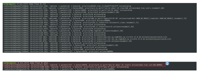
Now let us dump the flows on the integration bridge using ovs-ofctl dump-flows br-int. In the following image, I have marked those rules that are relevant for traffic coming from the instance.

IntegrationBridgeOutgoingRules

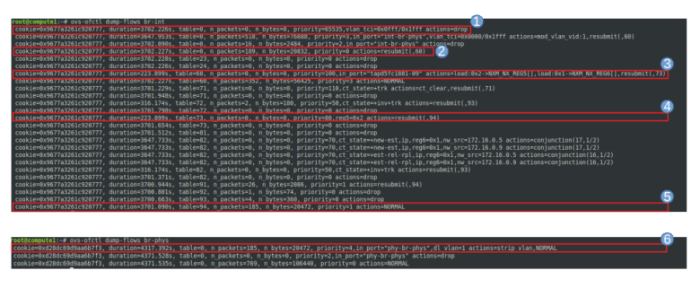
The first rule drops all traffic for which the VLAN TCI, masked with 0x1fff (i.e. the last 13 bits) is equal to 0x0fff, i.e. for which the VLAN ID is the reserved value 0xfff. These packets are assumed to be irregular and are dropped. The second rule directs all traffic coming from the tap device, i.e. from the virtual machine, to table 60.

In table 60, the traffic coming from the tap device, i.e. egress traffic, is marked by loading the registers 5 and 6, and resubmitted to table 73, where it is again resubmitted to table 94. In table 94, the packet is handed over to the ordinary switch processing using the NORMAL target.

When we dump the rules on the physical bridge br-phys, the result is much shorter and displayed in the lower part of the image above. Here, the first rule will pick up the traffic, strip off the VLAN tag (as expected) and hand it over to normal processing, so that the untagged package is forwarded to the physical network.

Let us now turn to the analysis of ingress traffic. If a packet arrives at br-phys, it is simply forwarded to br-int. Here, it is picked up by the second rule (unless it has a reserved VLAN ID) which adds a VLAN tag with ID 1 and resubmits to table 60. In this table, NORMAL processing is applied and the packet is forwarded to all ports. As the port connected to the tap device is an access port for VLAN 1, the packet is accepted by this port, the VLAN tag is stripped off again and the packet appears in the tap device and therefore in the virtual interface in the instance.

IntegrationBridgeIncomingRules

All this is a bit confusing but becomes clearer when we study the meaning of the various tables in the Neutron source code. The relevant source files are br_int.py and br_phys.py. Here is an extract of the relevant tables for the integration bridge from the code.

Table Name
0 Local switching table
23 Canary table
24 ARP spoofing table
25 MAC spoofing table
60 Transient table
71,72 Firewall for egress traffic
73,81,82 Firewall for accepted and ingress traffic
91 Accepted egress traffic
92 Accepted ingress traffic
93 Dropped traffic
94 Normal processing

Let us go through the meaning of some of these tables. The canary table (23) is simply used to verify that OVS is up and running (whence the name). The MAC spoofing and ARP spoofing tables (24, 25) are not populated in our example as we have disabled the port protection feature. Similarly, the firewall tables (71 , 72, 73, 81, 82) only contain a minimal setup. Table 91 (accepted egress traffic) simply routes to table 94 (normal processing), tables 92 and 93 are not used and table 94 simply hands over the packets to normal processing.

In our setup, the local switching table (table 0) and the transient table (table 60) are actually the most relevant tables. Together, these two tables realize the local VLANs on the compute node. We will see later that on each node, a local VLAN is built for each global virtual network. The method provision_local_vlan installs a rule into the local switching table for each local VLAN which adds the corresponding VLAN ID to ingress traffic coming from the corresponding global virtual and then resubmits to the transient table.

Here is the corresponding table for the physical bridge.

Table Name
0 Local switching table
2 Local VLAN translation

In our setup, only the local switching table is used which simply strips off the local VLAN tags for egress traffic.

You might ask yourself how we can reach the instances from the compute node. The answer is that a ping (or an SSH connection) to the instance running on the compute node actually travels via the default gateway, as there is no direct route to 172.16.0.0 on the compute node. In our setup, the gateway is 10.0.2.2 on the enp0s3 device which is the NAT-network provided by Virtualbox. From there, the connection travels via the lab host where we have configured the virtual network device vboxnet1 as a gateway for 172.16.0.0, so that the traffic enters the virtual network again via this gateway and eventually reaches enp0s9 from there.

We could now turn on port protection and security groups again and study the resulting rules, but this would go far beyond the scope of this post (and far beyond my understanding of OpenFlow rules). If you want to get into this, I recommend this summary of the firewall rules. Instead, we move on to a more complex setup using VLANs to separate virtual networks.

Adding a VLAN network

Let us now adjust our configuration so that we are able to provision a VLAN based virtual network. To do this, there are two configuration items that we have to change and that both appear in the configuration of the ML2 plugin.

The first item is type_drivers. Here, we need to add vlan as an additional value so that the VLAN type driver is loaded.

When starting up, this plugin loads the second parameter that we need to change – network_vlan_ranges. Here, we need to specify a list of physical network labels that can be used for VLAN based networks. In our case, we set this to physnet to use our only physical network that is connected via the br-phys bridge.

You can of course make these changes yourself (do not forget to restart the Neutron server) or you can use the Ansible scripts of lab 7. The demo script that is part of this lab will also create a virtual network based on VLAN ID 100 and attach two instances to it.

git clone https://github.com/christianb93/openstack-labs
cd openstack-labs/Lab7
vagrant up
ansible-playbook -i hosts.ini site.yaml
ansible-playbook -i hosts.ini demo.yaml

Once the instances are up, log again into the compute node and, as above, turn off port security for all ports. We can now go through the exercise above again and see what has changed.

First, ifconfig -a shows that the basic setup is the same as before. We have still our integration bridge connected to the tap device and connected to the physical bridge. Again, the port to which the tap device is attached is an access port, tagged with the VLAN ID 1. This is the local VLAN corresponding to our virtual network.

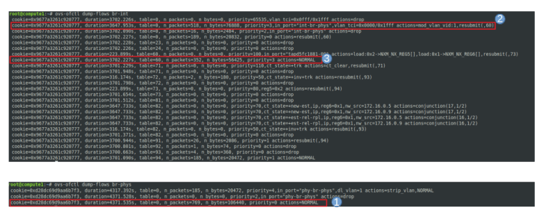
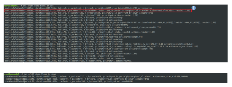
When we analyze the OpenFlow rules in the two bridges, however, a difference to our flat network is visible. Let us start again with egress traffic.

In the integration bridge, the flow is the same as before. As the port to which the VM is attached is an access port, traffic originating from the VM is tagged with VLAN ID 1, processed by the various tables and eventually forwarded via the virtual patch cable to br-phys.

Here, however, the handling is different. The first rule for this bridge matches, and the VLAN ID 1 is rewritten to become VLAN ID 100. Then, normal processing takes over, and the packet leaves the bridge and travels via enp0s9 to the physical network. Thus, traffic which the VLAN ID on the integration bridge shows up with VLAN ID 100 on the physical network. This is the mapping between local VLAN ID (which represents a virtual network on the node) and global VLAN ID (which represents a virtual VLAN network on the physical network infrastructure connecting the nodes).

IntegrationBridgeOutgoingRulesVLAN

For ingress traffic, the reverse mapping applies. A packet travels from the physical bridge to the integration bridge. Here, the second rule for table 0 matches for packets that are tagged with VLAN 100, the global VLAN ID of our virtual network, and rewrites the VLAN ID to 1, the local VLAN ID. This packet is then processed as before and eventually reaches the access port connecting the bridge with the tap device. There, the VLAN tagging is stripped off and the untagged traffic reaches the VM.

IntegrationBridgeIncomingRulesVLAN

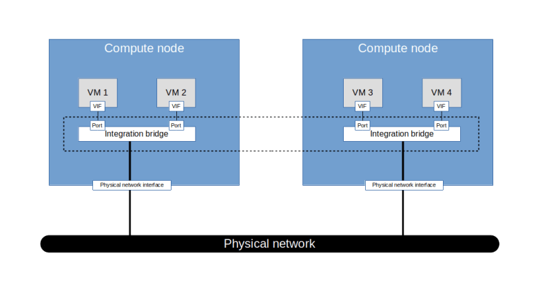
The diagram below summarizes our findings. We see that on the same physical infrastructure, two virtual networks are realized. There is still the flat network corresponding to untagged traffic, and the newly created virtual network corresponding to VLAN ID 100.

VLANNetworkTopology

It is interesting to note how the OpenFlow rules change if we bring up an additional instance on this compute node which is attached to the flat network. Then, an additional local VLAN ID (2 in our case) will appear corresponding to the flat network. On the physical bridge, the VLAN tag will be stripped off for egress traffic with this local VLAN ID, so that it appears untagged on the physical network. Similarly, on the integration bridge, untagged ingress traffic will no longer be dropped but will receive VLAN ID 2.

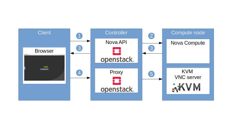
Note that this setup implies that we can no longer easily reach the machines connected to a VLAN network via SSH from the lab host or the compute node itself. In fact, even if we would set up a route to the vboxnet1 interface on the lab host, our traffic would come in untagged and would not reach the virtual machine. This is the reason why our lab 7 comes with a fully installed Horizon GUI which allows you to use the noVNC console to log into our instances.

This is very similar to a physical setup where a machine is connected to a switch via an access port, but the connection to the external network is on a different VLAN or on the untagged, native VLAN. In this situation, one would typically use a router to connect the two networks. Of course, Neutron offers virtual routers to connect two virtual networks. In the next post, we will see how this works and re-establish SSH connectivity to our instances.

OpenStack Neutron installation – basic setup and our first instances

In this post, we will go through the installation of Neutron for flat networks and get to know the basic configuration options for the various Neutron components, thus completing our first fully working OpenStack installation. If you have not already read my previous post describing some of the key concepts behind Neutron, I advise you to do this to be able to better follow todays post.

Installing Neutron on the controller node

The setup of Neutron on the controller node follows a similar logic to the installation of Nova or other OpenStack components that we have already seen. We create database tables and database users, add users, services and endpoints to Keystone, install the required packages, update the configuration and sync the database.

NeutronInstallation

As the first few steps are rather standard, let us focus on the configuration. There are

  • the Neutron server configuration file /etc/neutron.conf
  • the configuration of the ML2 plugin /etc/neutron/plugins/ml2/ml2_conf.ini
  • the configuration of the DHCP agent /etc/neutron/dhcp_agent.ini
  • the configuration of the DHCP agent /etc/neutron/metadata_agent.ini

Let us now discuss each of these configuration files in a bit more detail.

The Neutron configuration file on the controller node

The first group of options that we need to configure is familiar – the authorization strategy (keystone) and the related configuration for the Keystone authtoken middleware, the URL of the RabbitMQ server and the database connection as well as a directory for lock files.

The second change is the list of service plugins. Here we set this to an empty string, so that no additional service plugins beyond the core ML2 plugin will be loaded. At this point, we could configure additional services like Firewall-as-a-service which act as an extension.

Next we set the options notify_nova_on_port_status_changes and notify_nova_on_port_data_changes which instruct Neutron to inform Nova about status changes, for instance when the creation of a port fails.

To send these notifications, the external events REST API of Nova is used, and therefore Neutron needs credentials for the Nova service which need to be present in a section [nova] in the configuration file (loaded here).

The Neutron ML2 plugin configuration file

As you might almost guess from the presentation of Neutrons high-level architecture in the previous post, the ML2 plugin configuration file contains the information which type drivers and which mechanism drivers are loaded. The corresponding configuration items (type_drivers and mechanism_drivers) are both comma-separated lists. For our initial setup, we load the type drivers for a local network and a flat network, and we use the openvswitch mechanism driver.

In this file, we also configure the list of network types that are available as tenant networks. Here, we leave this list empty as we only offer a flat provider network.

In addition, we can configure so-called extension drivers. These are additional drivers that can be loaded by the ML2 plugin. In our case, the only driver that we load at this point in time is the port_security driver which allows us to disable the built-in port protection mechanisms and eases debugging.

In addition to the main [ml2] section, the configuration file also contains one section for each network type. As we only provide flat networks so far, we only have to populate this section. The parameter that we need is a list of flat networks. These networks are physical networks, but are not specified by the name of an actual physical interface, but by a logical network name which will later be mapped to an actual network device. Here, we choose the name physnet for our physical network.

The configuration of the metadata agent

We will talk in more detail about the metadata agent in a later post, and only briefly discuss it here. The metadata agent is an agent that allows instances to read metadata like the name of an SSH key using the de-facto standard provided by EC2s metadata service.

Nova provides a metadata API service that typically runs on a controller node. To allow access from within an instance, Neutron provides a proxy service which is protected by a secret shared between Nova and Neutron. In the configuration, we therefore need to provide the IP address (or DNS name) of the node on which the Nova metadata service is running and the shared secret.

The configuration of the DHCP agent

The configuration file for the DHCP agent requires only a few changes. First, we need to define the driver that the DHCP agent uses to connect itself to the virtual networks, which in our case is the openvswitch driver. Then, we need to specify the driver for the DHCP server itself. Here, we use the dnsmasq driver which actually spawns a dnsmasq process. We will learn more about DHCP agents in Neutron in a later post.

There is another feature that we enable in our configuration file. Our initial setup does not contain any router. Usually, routers are used to provide connectivity between an instance and the metadata service. To still allow the instances to access the metadata agent, the DHCP agent can be configured to add a static route to each instance pointing to the DHCP service. We enable this feature by setting the flag enable_isolated_metadata to true.

Installing Neutron on the compute nodes

We are now done with the setup of Neutron on the controller nodes and can turn our attention to the compute nodes. First, we need to install Open vSwitch and the neutron OVS agent on each compute node. Then, we need to create an OVS bridge on each compute node.

This is actually the point where I have been cheating in my previous post on Neutrons architecture. As mentioned there, Neutron does not connect the integration bridge directly to the network interface of the compute node. Instead, Neutron expects the presence of an additional OVS bridge that has to be provided by the adminstrator. We will simply let Neutron known what the name of this bridge is, and Neutron will attach it to the integration bridge and add a few OpenFlow rules. Everything else, i.e. how this bridge is connected to the actual physical network infrastructure, is up to the administrator. To create the bridge on the compute node, simply run (unless you are using my Ansible scripts, of course – see below)

ovs-vsctl  add-br br-int \
  -- set bridge br-int fail-mode=secure
ovs-vsctl add-port br-phys enp0s9

Once this is done, we now we need to adapt our configuration files as follows. In the item bridge_mappings, we need to provide the mapping from the physical network names to bridges. In our example, we have used the name physnet for our physical network. We now map this name to the device just created by setting

bridge_mappings = physnet:br-phys

We then need to define the driver that the Neutron agent uses to provide firewall functionality. This should of course be compatible with the chosen L2 driver, so we set this to openvswitch. We also enable security groups.

Once all configuration files have been updated, we should now restart the Neutron OVS agent on each compute node and all services on the controller nodes.

Installation using Ansible scripts

As always, I have put the exact steps to replicate this deployment into a set of Ansible scripts and roles. To run them, use (assuming, as always, that you did go through the basic setup described in an earlier post)

git clone https://github.com/christianb93/openstack-labs
cd openstack-labs/Lab5
vagrant up
ansible-playbook -i hosts.ini site.yaml

Let us now finally test our installation. We will create a project and a user, a virtual network, bring up two virtual machines, SSH into them and test connectivity.

First, we SSH into the controller node and source the OpenStack credentials for the admin user. We then create a demo project, assign the generated password for the demo user from demo-openrc, create the demo user with the corresponding password and assign the member role in the demo project to this user.

vagrant ssh controller
source admin-openrc
openstack project create demo
password=$(awk -F '=' '/OS_PASSWORD=/ { print $2}' demo-openrc)
openstack user create \
   --domain default\
   --project demo\
   --project-domain default\
   --password $password\
   demo
openstack role add \
   --user demo\
   --project demo\
   --project-domain default\
   --user-domain default member

Let us now create our network. This will be a flat network (the only type we have so far), based on the physical network physnet, and we will call this network demo-network.

openstack network create \
--share \
--external \
--provider-physical-network physnet \
--provider-network-type flat \
demo-network

Next, we create a subnet attached to this network with an IP range from 172.16.0.2 to 172.16.0.10.

openstack subnet create --network demo-network \
  --allocation-pool start=172.16.0.2,end=172.16.0.10 \
  --gateway 172.16.0.1 \
  --subnet-range 172.16.0.0/12 demo-subnet

Now we need to create a flavor. A flavor is a bit like a template for a virtual machines and defines the machine size.

openstack flavor create\
  --disk 1\
  --vcpus 1\
  --ram 512 m1.nano

To complete the preparations, we now have to adjust the firewall rules in the default security group to allow for ICMP and SSH traffic and to import the SSH key that we want to use. We execute these commands as the demo user.

source demo-openrc
openstack security group rule create --proto icmp default
openstack security group rule create --proto tcp --dst-port 22 default
openstack keypair create --public-key /home/vagrant/demo-key.pub demo-key

We are now ready to create our first instances. We will bring up two instances, called demo-instance-1 and demo-instance-2, both being attached to our demo network.

source demo-openrc
net_id=$(openstack network show -f value -c id demo-network)
openstack server create \
--flavor m1.nano \
--image cirros \
--nic net-id=$net_id \
--security-group default \
--key-name demo-key \
demo-instance-1
openstack server create \
--flavor m1.nano \
--image cirros \
--nic net-id=$net_id \
--security-group default \
--key-name demo-key \
demo-instance-2

To inspect the status of the instances, use openstack server list, which will also give you the IP address of the instances. To determine the IP address of the first demo instance and verify connectivity using ping, run

ip=$(openstack server show demo-instance-1 \
  -f value -c addresses \
  | awk -F "=" '{print $2}')
ping $ip

Finally, you should be able to SSH into your instances as follows.

ssh -i demo-key cirros@$ip

You can now ping the second instance and verify that the instance is in the ARP cache, demonstrating that there is a direct layer 2 connectivity between the instances.

We have now successfully completed a full OpenStack installation. In the next post, we will analyse the network setup that Neutron uses on the compute nodes in more detail. Until then, enjoy your running OpenStack playground!

OpenStack Neutron – architecture and overview

In this post, which is part of our series on OpenStack, we will start to investigate OpenStack Neutron – the OpenStack component which provides virtual networking services.

Network types and some terms

Before getting into the actual Neutron architecture, let us try to understand how Neutron provides virtual networking capabilities to compute instances. First, it is important to understand that in contrast to some container networking technologies like Calico, Neutron provides actual layer 2 connectivity to compute instances. Networks in Neutron are layer 2 networks, and if two compute instances are assigned to the same virtual network, they are connected to an actual virtual Ethernet segment and can reach each other on the Ethernet level.

What technologies do we have available to realize this? In a first step, let us focus on connecting two different virtual machines running on the same host. So assume that we are given two virtual machines, call them VM1 and VM2, on the same physical compute node. Our hypervisor will attach a virtual interface (VIF) to each of these virtual machines. In a physical network, you would simply connect these two interfaces to ports of a switch to connect the instances. In our case, we can use a virtual switch / bridge to achieve this.

OpenStack is able to leverage several bridging technologies. First, OpenStack can of course use the Linux bridge driver to build and configure virtual switches. In addition, Neutron comes with a driver that uses Open vSwitch (OVS). Throughout this series, I will focus on the use of OVS as a virtual switch.

So, to connect the VMs running on the same host, Neutron could use (and it actually does) an OVS bridge to which the virtual machine networking interfaces are attached. This bridge is called the integration bridge. We will see later that, as in a typical physical network, this bridge is also connected to a DHCP agent, routers and so forth.

NeutronNetworkingStepI

But even for the simple case of VMs on the same host, we are not yet done. In reality, to operate a cloud at scale, you will need some approach to isolate networks. If, for instance, the two VMs belong to different tenants, you do not want them to be on the same network. To do this, Neutron uses VLANs. So the ports connecting the integration bridge to the individual VMs are tagged, and there is one VLAN for each Neutron network.

This networking type is called a local network in Neutron. It is possible to set up Neutron to only use this type of network, but in reality, this is of course not really useful. Instead, we need to move on and connect the VMs that are attached to the same network on different hosts. To do this, we will have to use some virtual networking technology to connect the integration bridges on the different hosts.

NeutronNetworkingStepII

At this point, the above diagram is – on purpose – a bit vague, as there are several technologies available to achieve this (and I am cheating a bit and ignoring the fact that the integration bridge is not actually connected to a physical network interface but to a second bridge which in turn is connected to the network interface). First, we could simply connect each integration bridge to a physical network device which in turn is connected to the physical network. With this setup, called a flat network in Neutron, all virtual machines are effectively connected to the same Ethernet segment. Consequently, there can only be one flat network per deployment.

The second option we have is to use VLANs to partition the physical network according to the virtual networks that we wish to establish. In this approach, Neutron would assign a global VLAN ID to each virtual network (which in general is different from the VLAN ID used on the integration bridge) and tag the traffic within each virtual network with the corresponding VLAN ID before handing it over to the physical network infrastructure.

Finally, we could use tunnels to connect the integration bridges across the hosts. Neutron supports the most commonly used tunneling protocols (VXLAN, GRE, Geneve).

Regardless of the network type used, Neutron networks can be external or internal. External networks are networks that allow for connectivity to networks outside of the OpenStack deployment, like the Internet, whereas internal networks are isolated. Technically, Neutron does not really know whether a network has connectivity to the outside world, therefore “external network” is essentially a flag attached to a network which becomes relevant when we discuss IP routers in a later post.

Finally, Neutron deployment guides often use the terms provider network and tenant networks. To understand what this means, suppose you wanted to establish a network using e.g. VLAN tagging for separation. When defining this network, you would have to assign a VLAN tag to this virtual network. Of course, you need to make sure that there are no collisions with other Neutron networks or other reserved VLAN IDs on the physical networks. To achieve this, there are two options.

First, an administrator who has a certain understanding of the underlying physical network structure could determine an available VLAN ID and assign it. This implies that an administrator needs to define the network, and thus, from the point of view of a tenant using the platform, the network is created by the platform provider. Therefore, these networks are called provider networks.

Alternatively, an administrator could, initially, when installing Neutron, define a pool of available VLAN IDs. Using this pool, Neutron would then be able to automatically assing a VLAN ID when a tenant uses, say, the Horizon GUI to create a network. With this mechanism in place, tenants can define their own networks without having to rely on an administrator. Therefore, these networks are called tenant networks.

Neutron architecture

Armed with this basic understanding of how Neutron realizes virtual networks, let us now take a closer look at the architecture of Neutron.

NeutronArchitecture

The diagram above displays a very rough high-level overview of the components that make up Neutron. First, there is the Neutron server on the left hand side that provides the Neutron API endpoint. Then, there are the components that provide the actual functionality behind the API. The core functionality of Neutron is provided by a plugin called the core plugin. At the time of writing, there is one plugin – the ML2 plugin – which is provided by the Neutron team, but there are also other plugins available which are provided by third parties, like the Contrail plugin. Technically, a plugin is simply a Python class implementing the methods of the NeutronPluginBaseV2 class.

The Neutron API can be extended by API extensions. These extensions (which are again Python classes which are stored in a special directory and loaded upon startup) can be action extensions (which provide additional actions on existing resources), resource extensions (which provide new API resources) or request extensions that add new fields to existing requests.

Now let us take a closer look at the ML2 plugin. This plugin again utilizes pluggable modules called drivers. There are two types of drivers. First, there are type drivers which provide functionality for a specific network type, like a flat network, a VXLAN network, a VLAN network and so forth. Second, there are mechanism drivers that contain the logic specific to an implementation, like OVS or Linux bridging. Typically, the mechanism driver will in turn communicate with an L2 agent like the OVS agent running on the compute nodes.

On the right hand side of the diagram, we see several agents. Neutron comes with agents for additional functionality like DHCP, a metadata server or IP routing. In addition, there are agents running on the compute node to manipulate the network stack there, like the OVS agent or the Linux bridging agent, which correspond to the chosen mechanism drivers.

Basic Neutron objects

To close this post, let us take a closer look at same of the objects that Neutron manages. First, there are networks. As mentioned above, these are virtual layer 2 networks to which a virtual machine can attach. The point where the machine attaches is called a port. Each port belongs to a network and has a MAC address. A port contains a reference to the device to which it is attached. This can be a Nova managed instance, but also be another network device like a DHCP agent or a router. In addition, an IP address can be assigned to a port, either directly when the port is created (this is often called a fixed IP address) or dynamically.

In addition to layer 2 networks, Neutron has the concept of a subnet. A subnet is attached to a network and describes an IP network on top of this Ethernet network. Thus, a subnet has a CIDR and a gateway IP address.

Of course, this list is far from complete – there are routers, floating IP addresses, DNS servers and so forth. We will touch upon some of these objects in later posts in this series. In the next post, we will learn more about the components making up Neutron and how they are installed.

OpenStack Nova – deep-dive into the provisioning process

In the last post, we did go through the installation process and the high-level architecture of Nova, talking about the Nova API server, the Nova scheduler and the Nova agent. Today, we will make this a bit more tangible by observing how a typical request to provision an instance flows through this architecture.

The use case we are going to consider is the creation of a virtual server, triggered by a POST request to the /servers/ API endpoint. This is a long and complicated process, and we try to focus on the main path through the code without diving into every possible detail. This implies that we will skim over some points very briefly, but the understanding of the overall process should put us in a position to dig into other parts of the code if needed.

Roughly speaking, the processing of the request will start in the Nova API server which will perform validations and enrichments and populate the database. Then, the request is forwarded to the Nova conductor which will invoke the scheduler and eventually the Nova compute agent on the compute nodes. We will go through each of these phases in a bit more detail in the following sections.

Part I – the Nova API server

Being triggered by an API request, the process of course starts in the Nova API server. We have already seen in the previous post that the request is dispatched to a controller based on a set of hard-wired routes. For the endpoint in question, we find that the request is routed to the method create of the server controller.

This method first assembles some information like the user data which needs to be passed to the instance or the name of the SSH key to be placed in the instance. Then, authorization is carried out be calling the can method on the context (which, behind the scenes, will eventually invoke the Oslo policy rule engine that we have studied in our previous deep dive). Then the request data for networks, block devices and the requested image is processed before we eventually call the create method of the compute API. Finally, we parse the result and use a view builder to assemble a response.

Let us now see follow the call into the compute API. Here, all input parameters are validated and normalized, for instance by adding defaults. Then the method _provision_instances is invoked, which builds a request specification and the actual instance object and stores these objects in the database.

At this point, the Nova API server is almost done. We now call the method schedule_and_build_instances of the compute task API. From here, the call will simply be delegated to the corresponding method of the client side of the conductor RPC API which will send a corresponding RPC message to the conductor. At this point, we leave the Nova API server and enter the conductor. The flow through the code up to this point is summarized in the diagram below.

NovaProvisioningPartI

Part II – the conductor

In the last post, we have already seen that RPC calls are accepted by the Nova conductor service and are passed on to the Nova conductor manager. The corresponding method is schedule_and_build_instances

This method first retrieves the UUIDs of the instances from the request. Then, for each instance, the private method self._schedule_instances is called. Here, the class SchedulerQueryClient is used to submit an RPC call to the scheduler, which is being processed by the schedulers select_destinations method.

We will not go into the details of the scheduling process here, but simply note that this will in turn make a call to the placement service to retrieve allocation candidates and then calls the scheduler driver to actually select a target host.

Back in the conductor, we check whether the scheduling was successful. It not, the instance is moved into the cell0. If yes, we determine the cell in which the selected host is living, update some status information and eventually, at the end of the method, invoke the method build_and_run_instance of the RPC client for the Nova compute service. At this point, we leave the Nova conductor service and the processing continues in the Nova compute service running on the selected host.

InstanceCreationPartII

Part III – the processing on the compute node

We have now reached the Nova compute agent running on the selected compute node, more precisely the method build_and_run_instance of the Nova compute manager. Here we spawn a separate worker thread which runs the private method _do_build_and_run_instance.

This method updates the VM state to BUILDING and calls _build_and_run_instance. Within this method, we first invoke _build_resources which triggers the creation of resources like networks and storage devices, and then move on to the spawn method of the compute driver from nova.virt. Note that this is again a pluggable driver mechanism – in fact the compute driver class is an abstract class, and needs to be implemented by each compute driver.

Now let us see how the processing works in our specific case of the libvirt driver library. First, we create an image for the VM by calling the private method _create_image. Next, we create the XML descriptor for the guest, i.e. we retrieve the required configuration data and turn it into the XML structure that libvirt expects. Finally, we call _create_domain_and_network and finally set a timer to periodically check the state of the instance until the boot process is complete.

In _create_domain_and_network, we plug in the virtual network interfaces, set up the firewall (in our installation, this is the point where we use the No-OP firewall driver as firewall functionality is taken over by Neutron) and then call _create_domain which creates the actual guest (called a domain in libvirt).

This delegates the call to nova.virt.libvirt.Guest.create()and then powers on the guest using the launch method on the newly created guest. Let us take a short look at each of these methods in turn.

In nova.virt.libvirt.Guest.create(), we use the write_instance_config method of the host class to create the libvirt guest without starting it.

In the launch method in nova/virt/libvirt/guest.py, we now call createWithFlags on the domain. This is actually a call into the libvirt library itself and will launch the previously defined guest.

InstanceCreationPartIII

At this point, our newly created instance will start to boot. The timer which we have created earlier will check in periodic intervalls whether the boot process is complete and update the status of the instance in the database accordingly.

This completes our short tour through the instance creation process. There are a few points which we have deliberately skipped, for instance the details of the scheduling process, the image creation and image caching on the compute nodes or the network configuration, but the information in this post might be a good starting point for further deep dives.

OpenStack Nova – installation and overview

In this post, we will look into Nova, the cloud fabric component of OpenStack. We will see how Nova is installed and go briefly through the individual components and Nova services.

Overview

Before getting into the installation process, let us briefly discuss the various components of Nova on the controller and compute nodes.

First, there is the Nova API server which runs on the controller node. The Nova service will register itself as a systemd service with entry point /usr/bin/nova-api. Similar to Glance, invoking this script will bring up an WSGI server which uses PasteDeploy to build a pipeline with the actual Nova API endpoint (an instance of nova.api.openstack.compute.APIRouterV21) being the last element of the pipeline. This component will then distribute incoming API requests to various controllers which are part of the nova.api.openstack.compute module. The routing rules themselves are actually hardcoded in the ROUTE_LIST which is part of the Router class and maps request paths to controller objects and their methods.

NovaAPIComponents

When you browse the source code, you will find that Nova offers some APIs like the image API or the bare metal API which are simply proxies to other OpenStack services like Glance or Ironic. These APIs are deprecated, but still present for backwards compatibility. Nova also has a network API which, depending on the value of the configuration item use_neutron will either acts as proxy to Neutron or will present the legacy Nova networking API.

The second Nova component on the controller node is the Nova conductor. The Nova conductor does not expose a REST API, but communicates with the other Nova components via RPC calls (based on RabbitMQ). The conductor is used to handle long-running tasks like building an instance or performing a live migration.

Similar to the Nova API server, the conductor has a tiered architecture. The actual binary which is started by the systemd mechanism creates a so called service object. In Nova, a service objects represents an RPC API endpoint. When a service object is created, it starts up an RPC service that handles the actual communication via RabbitMQ and forwards incoming requests to an associated service manager object.

NovaRPCAPI

Again, the mapping between binaries and manager classes is hardcoded and, for the Stein release, is as follows.

SERVICE_MANAGERS = {
  'nova-compute': 'nova.compute.manager.ComputeManager',
  'nova-console': 'nova.console.manager.ConsoleProxyManager',
  'nova-conductor': 'nova.conductor.manager.ConductorManager',
  'nova-metadata': 'nova.api.manager.MetadataManager',
  'nova-scheduler': 'nova.scheduler.manager.SchedulerManager',
}

Apart from the conductor service, this list contains one more component that runs on the controller node and use the same mechanism to handle RPC requests (the nova-console binary is deprecated and we use the noVNC proxy, see the section below, the nova-compute binary is running on the compute node, and the nova-metadata binary is the old metadata service used with the legacy Nova networking API). This is the the Nova scheduler.

The scheduler receives and maintains information on the instances running on the individual hosts and, upon request, uses the Placement API that we have looked at in the previous post to take a decision where a new instance should be placed. The actual scheduling is carried out by a pluggable instance of the nova.scheduler.Scheduler base class. The default scheduler is the filter scheduler which first applies a set of filters to filter out individual hosts which are candidates for hosting the instance, and then computes a score using a set of weights to take a final decision. Details on the scheduling algorithm are described here.

The last service which we have not yet discussed is Nova compute. One instance of the Nova compute service runs on each compute node. The manager class behind this service is the ComputeManager which itself invokes various APIs like the networking API or the Cinder API to manage the instances on this node. The compute service interacts with the underlying hypervisor via a compute driver. Nova comes with compute driver for the most commonly used hypervisors, including KVM (via libvirt), VMWare, HyperV or the Xen hypervisor. In a later post, we will go once through the call chain when provisioning a new instance to see how the Nova API, the Nova conductor service, the Nova compute service and the compute driver interact to bring up the machine.

The Nova compute service itself does not have a connection to the database. However, in some cases, the compute service needs to access information stored in the database, for instance when the Nova compute service initializes on a specific host and needs to retrieve a list of instances running on this host from the database. To make this possible, Nova uses remotable objects provided by the Oslo versioned objects library. This library provides decorators like remotable_classmethod to mark methods of a class or an object as remotable. These decorators point to the conductor API (indirection_api within Oslo) and delegate the actual method invocation to a remote copy via an RPC call to the conductor API. In this way, only the conductor needs access to the database and Nova compute offloads all database access to the conductor.

Nova cells

In a large OpenStack installation, access to the instance data stored in the MariaDB database can easily become a bottleneck. To avoid this, OpenStack provides a sharding mechanism for the database known as cells.

The idea behind this is that the set of your compute nodes are partitioned into cells. Every compute node is part of a cell, and in addition to these regular cells, there is a cell called cell0 (which is usually not used and only holds instances which could not be scheduled to a node). The Nova database schema is split into a global part which is stored in a database called the API database and a cell-local part. This cell-local database is different for each cell, so each cell can use a different database running (potentially) on a different host. A similar sharding applies to message queues. When you set up a compute node, the configuration of the database connection and the connection to the RabbitMQ service determine to which cell the node belongs. The compute node will then use this database connection to register itself with the corresponding cell database, and a special script (nova-manage) needs to be run to make these hosts visible in the API database as well so that they can be used by the scheduler.

Cells themselves are stored in a database table cell_mappings in the API database. Here each cell is set up with a dedicated RabbitMQ connection string (called the transport URL) and a DB connection string. Our setup will have two cells – the special cell0 which is always present and a cell1. Therefore, our installation will required three databases.

Database Description
nova_api Nova API database
nova_cell0 Database for cell0
nova Database for cell1

In a deployment with more than one real cell, each cell will have its own Nova conductor service, in addition to a “super conductor” running across cells, as explained here and in diagram below which is part of the OpenStack documentation.

The Nova VNC proxy

Usually, you will use SSH to access your instances. However, sometimes, for instance if the SSHD is not coming up properly or the network configuration is broken, it would be very helpful to have a way to connect to the instance directly. For that purpose, OpenStack offers a VNC console access to running instances. Several VNC clients can be used, but the default is to use the noVNC browser based client embedded directly into the Horizon dashboard.

How exactly does this work? First, there is KVM. The KVM hypervisor has the option to export the content of the emulated graphics card of the instance as a VNC server. Obviously, this VNC server is running on the compute node on which the instance is located. The server for the first instance will listen on port 5900, the server for the second instance will listen on port 5901 and so forth. The server_listen configuration option determines the IP address to which the server will bind.

Now theoretically a VNC client like noVNC could connect directly to the VNC server. However, in most setups, the network interfaces of the compute node are not directly reachable from a browser in which the Horizon GUI is running. To solve this, Nova comes with a dedicated proxy for noVNC. This proxy is typically running on the controller node. The IP address and port number on which this proxy is listening can again be configured using the novncproxy_host and novncproxy_port configuration items. The default port is 6080.

When a client like the Horizon dashboard wants to get access to the proxy, it can use the Nova API path /servers/{server_id}/remote-consoles. This call will be forwarded to the Nova compute method get_vnc_console on the compute node. This method will return an URL, consisting of the base URL (which can again be configured using the novncproxy_base_url configuration item), and a token which is stored in the database as well. When the client uses this URL to connect to the proxy, the token is used to verify that the call is authorized.

The following diagram summarizes the process to connect to the VNC console of an instance from a browser running noVNC.

NoVNCProxy

  1. Client uses Nova API /servers/{server_id}/remote-consoles to retrieve the URL of a proxy
  2. Nova API delegates the request to Nova Compute on the compute node
  3. Nova Compute assembles the URL, which points to the proxy, and creates a token, containing the ID of the instance as well as additional information, and the URL including the token is handed out to the client
  4. Client uses the URL to connect to the proxy
  5. The proxy validates the token, extracts the target compute node and port information, establishes the connection to the actual VNC server and starts to service the session

Installing Nova on the controller node

Armed with the knowledge from the previous discussions, we can now almost guess what steps we need to take in order to install Nova on the controller node.

NovaInstallation

First, we need to create the Nova databases – the Nova API database (nova_api), the Nova database for cell0 (nova_cell0) and the Nova database for our only real cell cell1 (nova). We also need to create a user which has the necessary grants on these databases.

Next, we create a user in Keystone representing the Nova service, register the Nova API service with Keystone and define endpoints.

We then install the Ubuntu packages corresponding to the four components that we will install on the controller node – the Nova API service, the Nova conductor, the Nova scheduler and the VNC proxy.

Finally, we adapt the configuration file /etc/nova/nova.conf. The first change is easy – we set the value my_ip to the IP of the controller management interface.

We then need to set up the networking part. To enforce the use of Neutron instead of the built-in legacy Nova networking, we set the configuration option use_neutron that we already discussed above to True. We also set the firewall driver to the No-OP driver nova.virt.firewall.NoopFirewallDriver.

The next information we need to provide is the connection information to RabbitMQ and the database. Recall that we need to configure two database connections, one for the API database and one for the database for cell 1 (Nova will automatically append _cell0 to this database name to obtain the database connection for cell 0).

We also need to provide some information that Nova needs to communicate with other Nova services. In the glance section, we need to define the URL to reach the Glance API server. In the neutron section, we need to set up the necessary credentials to connect to Neutron. Here we use a Keystone user neutron which we will set up when installing Neutron in a later post, and we also define some data needed for the metadata proxy that we will discuss in a later post. And finally Nova needs to connect to the Placement service for which we have to provide credentials as well, this time using the placement user created earlier.

To set up the communication with Keystone, we need to set the authorization strategy to Keystone (which will also select the PasteDeploy Pipeline containing the Keystone authtoken middleware) and provide the credentials that the authtoken middleware needs. And finally, we set the path that the Oslo concurrency library will use to create temporary files.

Once all this has been done, we need to prepare the database for use. As with the other services, we need to sync the database schema to the latest version which, in our case, will simply create the database schema from scratch. We also need to establish our cell 1 in the database using the nova-manage utility.

Installing Nova on the compute nodes

Let us now turn to the installation of Nova on the compute nodes. Recall that on the compute nodes, only nova-compute needs to be running. There is no database connection needed, so the only installation step is to install the nova-compute package and to adapt the configuration file.

The configuration file nova.conf on the compute node is very similar to the configuration file on the controller node, with a few differences.

As there is no database connection, we can comment out the DB connection string. In the light of our above discussion of the VNC proxy mechanism, we also need to provide some configuration items for the proxy mechanism.

  • The configuration item server_proxyclient_address is evaluated by the get_vnc_console of the compute driver and used to return the IP and port number on which the actual VNC server is running and can be reached from the controller node (this is the address to which the proxy will connect)
  • The server_listen configuration item is the IP address to which the KVM VNC server will bind on the compute host and should be reachable via the server_proxyclient_address from the controller node
  • the novncproxy_base_url is the URL which is handed out by the compute node for use by the proxy

Finally, there is a second configuration file nova-compute.conf specific to the compute nodes. This file determines the compute driver used (in our case, we use libvirt) and the virtualization type. With libvirt, we can either use KVM or QEMU. KVM will only work if the CPU supports virtualization (i.e. offers the VT-X extension for Intel or AMD-V for AMD). In our setup, the virtual machines will run on top of another virtual machine (Virtualbox), which does only pass through these features for AMD CPUs. We will therefore set the virtualization type to QEMU.

Finally, after installing Nova on all compute nodes, we need to run the nova-manage tool once more to make these nodes known and move them into the correct cells.

Run and verify the installation

Let us now run the installation and verify that is has succeeded. Here are the commands to bring up the environment and to obtain and execute the needed playbooks.

git clone https://www.github.com/christianb93/openstack-labs
cd openstack-labs/Lab4
vagrant up
ansible-playbook -i hosts.ini site.yaml

This will run a few minutes, depending on the network connection and the resources available on your machine. Once the installation completes, log into the controller and source the admin credentials.

vagrant ssh controller
source admin-openrc

First, we verify that all components are running on the controller. To do this, enter

systemctl | grep "nova"

The output should contain four lines, corresponding to the four services nova-api, nova-conductor, nova-scheduler and nova-novncproxy running on the controller node. Next, let us inspect the Nova database to see which compute services have registered with Nova.

openstack compute service list

The output should be similar to the sample output below, listing the scheduler, the conductor and two compute instances, corresponding to the two compute nodes that our installation has.

+----+----------------+------------+----------+---------+-------+----------------------------+
| ID | Binary         | Host       | Zone     | Status  | State | Updated At                 |
+----+----------------+------------+----------+---------+-------+----------------------------+
|  1 | nova-scheduler | controller | internal | enabled | up    | 2019-11-18T08:35:04.000000 |
|  6 | nova-conductor | controller | internal | enabled | up    | 2019-11-18T08:34:56.000000 |
|  7 | nova-compute   | compute1   | nova     | enabled | up    | 2019-11-18T08:34:56.000000 |
|  8 | nova-compute   | compute2   | nova     | enabled | up    | 2019-11-18T08:34:57.000000 |
+----+----------------+------------+----------+---------+-------+----------------------------+

Finally, the command sudo nova-status upgrade check will run some checks meant to be executed after an update that can be used to further verify the installation.

OpenStack supporting services – Glance and Placement

Apart from Keystone, Glance and Placement are two additional infrastructure services that are part of every OpenStack installation. While Glance is responsible for storing and maintaining disk images, Placement (formerly part of Nova) is keeping track of resources and allocation in a cluster.

Glance installation

Before we get into the actual installation process, let us take a short look at the Glance runtime environment. Different from Keystone, but similar to most other OpenStack services, Glance is not running inside Apache, but is an independent process using a standalone WSGI server.

To understand the startup process, let us start with the setup.cfg file. This file contains an entry point glance-api which, via the usual mechanism provided by Pythons setuptools, will provide a Python executable which runs glance/cmd/api.py. This in turn uses the simple WSGI server implemented in glance/common/wsgi.py. This server is then started in the line

server.start(config.load_paste_app('glance-api'), default_port=9292)

Here we see that the actual WSGI app is created and passed to the server using the PasteDeploy Python library. If you have read my previous post on WSGI and WSGI middleware, you will know that this is a library which uses configuration data to plumb together a WSGI application and middleware. The actual call of the PasteDeploy library is delegated to a helper library in glance/common and happens in the function load_past_app defined here.

Armed with this understanding, let us now dive right into the installation process. We will spend a bit more time with this process, as it contains some recurring elements which are relevant for most of the OpenStack services that we will install and use. Here is a graphical overview of the various steps that we will go through.

GlanceInstallationProcess

The first thing we have to take care of is the database. Almost all OpenStack services require some sort of database access, thus we have to create one or more databases in our MariaDB database server. In the case of Glance, we create a database called glance. To allow Glance to access this database, we also need to set up a corresponding MariaDB user and grant the necessary access rights on our newly created database.

Next, Glance of course needs access to Keystone to authenticate users and authorize API requests. For that purpose, we create a new user glance in Keystone. Following the recommended installation process, we will in fact create one Keystone user for every OpenStack service, which is of course not strictly necessary.

With this, we have set up the necessary identities in Keystone. However, recall that Keystone is also used as a service catalog to decouple services from endpoints. An API user will typically not access Glance directly, but first get a list of service endpoints from Keystone, select an appropriate endpoint and then use this endpoint. To support this pattern, we need to register Glance with the Keystone service catalog. Thus, we create a Keystone service and API endpoints. Note that the port provided needs to match the actual port on which the Glance service is listening (using the default unless overridden explicitly in the configuration).

OpenStack services typically expose more than one endpoint – a public endpoint, an internal endpoint and an admin endpoint. As described here, there does not seem to be fully consistent configuration scheme that allows an administrator to easily define which endpoint type the services will use. Following the installation guideline, we will install all our services with all three endpoint types.

Next, we can install Glance by simply installing the corresponding APT package. Similar to Keystone, this package comes with a set of configuration files that we now have to adapt.

The first change which is again standard across all OpenStack components is to change the database connection string so that Glance is able to find our previously created database. Note that this string needs to contain the credentials for the Glance database user that we have created.

Next, we need to configure the Glance WSGI middleware chain. As discussed above, Glance uses the PasteDeploy mechanism to create a WSGI application. When you take a look at the corresponding configuration, however, you will see that it contains a variety of different pipeline definitions. To select the pipeline that will actually be deployed, Glance has a configuration option called deployment flavor. This is a short form for the name of the pipeline to be selected, and when the actual pipeline is assembled here, the name of the pipeline is put together by combining the flavor with the string “glance-api”. We use the flavor “keystone” which will result in the pipeline “glance-api-keystone” being loaded.

This pipeline contains the Keystone auth token middleware which (as discussed in our deep dive into tokens and policies) extracts and validates the token data in a request. This middleware components needs access to the Keystone API, and therefore we need to add the required credentials to our configuration in the section [keystone_authtoken].

To complete the installation, we still have to create the actual database schema that Glance expects. Like most other OpenStack services, Glance is able to automatically create this schema and to synchronize an existing database with the current version of the existing schema by automatically running the necessary migration routines. This is done by the helper script glance-manage.

The actual installation process is now completed, and we can restart the Glance service so that the changes in our configuration files are picked up.

Note that the current version of the OpenStack install guide for Stein will instruct you to start two Glance services – glance-api and glance-registry. We only start the glance-api service, for the following reason.

Internally, Glance is structured into a database access layer and the actual Glance API server, plus of course a couple of other components like common services. Historically, Glance used the first of todays three access layers called the Glance registry. Essentially, the Glance registry is a service sitting between the Glance API service and the database, and contains the code for the actual database layer which uses SQLAlchemy. In this setup, the Glance API service is reachable via the REST API, whereas the Glance registry server is only reachable via RPC calls (using the RabbitMQ message queue). This will add an additional layer of security, as the database credentials need to be stored in the configuration of the Glance registry service only, and makes it easier to scale Glance across several nodes. Later, the Glance registry service was deprecated, and the actual configuration instructs Glance to access the database directly (this is the data_api parameter in the Glance configuration file).

As in my previous posts, I will not replicate the exact commands to do all this manually (you can find them in the well-written OpenStack installation guide), but have put together a set of Ansible scripts doing all this. To run them, enter the following commands

git clone https://github.com/christianb93/openstack-labs
cd Lab3
vagrant up
ansible-playbook -i hosts.ini site.yaml

This playbook will not only install and configure the Glance service, but will also download the CirrOS image (which I have mirrored in an S3 bucket as the original location is sometimes a bit slow) and import it into Glance.

Working with Glance images

Let us now play a bit with Glance. The following commands need to be run from the controller node, and we have to source the credentials that we need to connect to the API. So SSH into the controller node and source the credentials by running

vagrant ssh controller
source admin-openrc

First, let us use the CLI to display all existing images.

openstack image list

As we have only loaded one image so far – the CirrOS image – the output will be similar to the following sample output.

+--------------------------------------+--------+--------+
| ID                                   | Name   | Status |
+--------------------------------------+--------+--------+
| f019b225-de62-4782-9206-ed793fbb789f | cirros | active |
+--------------------------------------+--------+--------+

Let us now get some more information on this image. For better readability, we display the output in JSON format.

openstack image show cirros -f json

The output is a bit longer, and we will only discuss a few of the returned attributes. First, there is the file attribute. If you look at this and compare this to the contents of the directory /var/lib/glance/images/, you will see that this is a reference to the actual image stored on the hard disk. Glance delegates the actual storage to a storage backend. Storage backends are provided by the separate glance_store library and include a file store (which simply stores files on the disk as we have observed and is the default), a HTTP store which uses a HTTP GET to retrieve an image, an interface to the RADOS distribute object store and interfaces to Cinder, Swift and VMWare data store.

We also see from the output that images can be active or inactive, belong to a project (the owner field refers to a project), can be tagged and can either be visible for the public (i.e. outside the project to which they belong) or private (i.e. only visible within the project). It is also possible to share images with individual projects by adding these projects as members.

Note that Glance stores image metadata, like visibility, hash values, owner and so forth in the database, while the actual image is stored in one of the storage backends.

Let us now go through the process of adding an additional image. The OpenStack Virtual Machine Image guide contains a few public sources for OpenStack images and explains how adminstrators can create their own images based on the most commonly used Linux distributions. As an example, here are the commands needed to download the latest Ubuntu Bionic cloud image and import it into Glance.

wget http://cloud-images.ubuntu.com/bionic/current/bionic-server-cloudimg-amd64.img
openstack image create \
    --disk-format qcow2 \
    --file bionic-server-cloudimg-amd64.img \
    --public \
    --project admin \
    ubuntu-bionic

We will later see how we need to reference an image when creating a virtual machine.

Installing the placement service

Having discussed the installation process for the Glance service in a bit more detail, let us now quickly go over the steps to install Placement. Structurally, these steps are almost identical to those to install Glance, and we will not go into them in detail.

PlacementInstallation

Also the changes in the configuration file are very similar to those that we had to apply for Glance. Placement again uses the Keystone authtoken plugin, so that we have to supply credentials for Keystone in the keystone_authtoken section of the configuration file. We also have to supply a database connection string. Apart from that, we can take over the default values in the configuration file without any further changes.

Placement overview

Let us now investigate the essential terms and objects that the Placement API uses. As the openstack client does not yet contain full support for placement, we will directly use the API using curl. With each request, we need to include two header parameters.

  • X-Auth-Token needs to contain a valid token that we need to retrieve from Keystone first
  • OpenStack-API-Version needs to be included to define the version of the API (this is the so-called microversion).

Here is an example. We will SSH into the controller, source the credentials, get a token from Keystone and submit a GET request on the URL /resource_classes that we feed into jq for better readability.

vagrant ssh controller
source admin-openrc
sudo apt-get install jq
token=$(openstack token issue -f json | jq -r ".id") 
curl \
  -H "X-Auth-Token: $token" \
  -H "OpenStack-API-Version: placement 1.31"\
  "http://controller:8778/resource_classes" | jq

The resulting list is a list of all resource classes known to Placement. Resource classes are types of resources that Placement manages, like IP addresses, vCPUs, disk space or memory. In a fully installed system, OpenStack services can register as resource providers. Each provider offers a certain set of resource classes, which is called an inventory. A compute node, for instance, would typically provide CPUs, disk space and memory. In our current installation, we cannot yet test this, but in a system with compute nodes, the inventory for a compute node would typically look as follows.

{
  "resource_provider_generation": 3,
  "inventories": {
    "VCPU": {
      "total": 2,
      "reserved": 0,
      "min_unit": 1,
      "max_unit": 2,
      "step_size": 1,
      "allocation_ratio": 16
    },
    "MEMORY_MB": {
      "total": 3944,
      "reserved": 512,
      "min_unit": 1,
      "max_unit": 3944,
      "step_size": 1,
      "allocation_ratio": 1.5
    },
    "DISK_GB": {
      "total": 9,
      "reserved": 0,
      "min_unit": 1,
      "max_unit": 9,
      "step_size": 1,
      "allocation_ratio": 1
    }
  }
}

Here we see that the compute node has two virtual CPUs, roughly 4 GB of memory and 9 GB of disk space available. For each resource provider, Placement also maintains usage data which keeps track of the current usage of the resources. Here is a JSON representation of the usage for a compute node.

{
  "resource_provider_generation": 3,
  "usages": {
    "VCPU": 1,
    "MEMORY_MB": 128,
    "DISK_GB": 1
  }
}

So in this example, one vCPU, 128 MB RAM and 1 GB disk of the compute node are in use. To link consumers and usage information, Placement uses allocations. An allocation represents a usage of resources by a specific consumer, like in the following example.

{
  "allocations": {
    "aaa957ac-c12c-4010-8faf-55520200ed55": {
      "resources": {
        "DISK_GB": 1,
        "MEMORY_MB": 128,
        "VCPU": 1
      },
      "consumer_generation": 1
    }
  },
  "resource_provider_generation": 3
}

In this case, the consumer (represented by the UUID aaa957ac-c12c-4010-8faf-55520200ed55) is actually a compute instance which consumes 1 vCPU, 128 MB memory and 1 GB disk space. Here is a diagram that represents a simplified version of the Placement data model.

PlacementDataModel

Placement offers a few additional features like Traits, which define qualitative properties of resource providers, or aggregates which are groups of resource providers, or the ability to make reservations.

Let us close this post by briefly discussing the relation between Nova and Placement. As we have mentioned above, compute nodes represent resource providers in Placement, so Nova needs to register resource provider records for the compute nodes it manages and providing the inventory information. When a new instance is created, the Nova scheduler will request information on inventories and current usage from Placement to determine the compute node on which the instance will be placed, and will subsequently update the allocations to register itself as a consumer for the resources consumed by the newly created instance.

With this, the installation of Glance and Placement is complete and we have all the ingredients in place to start installing the Nova services in the next post.

OpenStack Keystone – a deep-dive into tokens and policies

In the previous post, we have installed Keystone and provided an overview of its functionality. Today, we will dive in detail into a typical authorization handshake and take you through the Keystone source code to see how it works under the hood.

The overall workflow

Let us first take a look at the overall process before we start to dig into details. As an example, we will use the openstack CLI to list all existing projects. To better see what is going on behind the scenes, we run the openstack client with the -v command line switch which creates a bit more output than usual.

So, log into the controller node and run

source admin-demorc
openstack -vv project list

This will give a rather lengthy output, so let us focus on those lines that signal that a requests to the API is made. The first API is a GET request to the URL

http://controller:5000/v3

This request will return a list of available API versions, marked with a status. In our case, the result indicates that the stable version is version v3. Next, the clients submits a POST request to the URL

http://controller:5000/v3/auth/tokens

If we look up this API endpoint in the Keystone Identity API reference, we find that this method is used to create and return a token. When making this request, the client will use the data provided in the environment variables set by our admin-openrc script to authenticate with Keystone, and Keystone will assemble and return a token.

The returned data has actually two parts. First, there is the actual Fernet token, which is provided in the HTTP header instead of the HTTP body. Second, there is a token structure which is returned in the response body. This structure contains the user that owns the token, the date when the token expires and the data when the token has been issued, the project for which the token is valid (for a project scoped token) and the roles that the user has for this project. In addition, it contains a service catalog. Here is an example, where I have collapsed the catalog part for better readibility.

token

Finally, at the bottom of the output, we see that the actual API call to get a list of projects is made, using our newly acquired token and the endpoint

http://controller:5000/v3/projects

So our overall flow looks like this, ignoring some client internal processes like selecting the endpoint (and recovering from failed authorizations, see the last section of this post).

AuthorizationWorkflowGetProjects

Let us now go through these requests step by step and see how tokens and policies interact.

Creating a token

When we submit the API request to create a token, we end up in the method post in the AuthTokenResource class defined in keystone/api/auth.py. Here we find the code.

token=authentication.authenticate_for_token(auth_data)
resp_data=render_token.render_token_response_from_model(
          token, include_catalog=include_catalog
)

The method authenticate_for_token is defined in keystone/api/_shared/authentication.py. Here, we first authenticate the user, using the auth data provided in the request, in our case this is username, password, domain and project as defined in admin-openrc. Then, the actual token generation is triggered by the call

token=PROVIDERS.token_provider_api.issue_token(
          auth_context['user_id'], 
          method_names, 
          expires_at=expires_at,
          system=system, 
          project_id=project_id, 
          domain_id=domain_id,
          auth_context=auth_context, 
          trust_id=trust_id,
          app_cred_id=app_cred_id, 
         parent_audit_id=token_audit_id)

Here we see an additional layer of indirection in action – the ProviderAPIRegistry as defined in keystone/common/provider_api.py. Without getting into details, here is the idea of this approach which is used in a similar way in other OpenStack services.

Keystone itself consists of several components, each of which provide different methods (aka internal APIs). There is, for instance, the code in keystone/identity handling the core identity features, the code in keystone/assignment handling role assigments, the code in keystone/token handling tokens and so forth. Each of these components contains a class typically called Manager which is derived from the base class Manager in keystone/common/manager.py.

When such a class is instantiated, it registers its methods with the static instance ProviderAPI of the class ProviderAPIRegistry defined in keystone/common/provider_api.py. Technically, registering means that the object is added as attribute to the ProviderAPI object. For the token API, for instance, the the Manager class in keystone/token/provider.py registers itself using the name token_provider_api, so that it is added to the provider registry object as the attribute token_provider_api. Thus a method XXX of this manager class can now be invoked using

from keystone.common import provider_api
provider_api.ProviderAPIs.token_provider_api.XXX()

or by

from keystone.common import provider_api
PROVIDERS = provider_api.ProviderAPIs
PROVIDERS.token_provider_api.XXX()

This is exactly what happens here, and this is why the above line will actually take us to the method issue_token of the Manager class defined in keystone/token/provider.py. Here, we build and populate an instance of the Token class defined in keystone/models/token_model.py and populate it with the available data. We then populate the field token.id where we put the actual token, i.e. the encoded string that will end up in the HTTP header of future requests. This is done in the line

token_id, issued_at =
             self.driver.generate_id_and_issued_at(token)

which calls the actual token provider, for instance the Fernet provider. For a Fernet token, this will eventually end up in the line

token_id=self.token_formatter.create_token(
    token.user_id,
    token.expires_at,
    token.audit_ids,
    token_payload_class,
    methods=token.methods,
    system=token.system,
    domain_id=token.domain_id,
    project_id=token.project_id,
    trust_id=token.trust_id,
    federated_group_ids=token.federated_groups,
    identity_provider_id=token.identity_provider_id,
    protocol_id=token.protocol_id,
    access_token_id=token.access_token_id,
    app_cred_id=token.application_credential_id
)

calling the token formatter which will do the low level work of actually creating and encrypting the token. The token ID will then be added to the token data structure, along with the creation time (a process known as minting) before the token is returned up the call chain.

At this point, the token does not yet contain any role information and no service catalog. To enrich the token by this information, it is rendered by calling render_token defined in keystone/common/render_token.py. Here, a dictionary is built and populated with data including information on role, scope and endpoints.

Note that the role information in the token is dynamic, in fact, in the Token class, the property decoration is used to divert access to the roles property to a method call. Here, we receive the scope information and select and return only these roles which are bound to the respective domain or project if the token is domain scoped or project scoped. When we render the token, we access the roles attribute and retrieve the role information from the method bound to it.

Within this method, an additional piece of logic is implemented which is relevant for the later authorization process. Keystone allows an administrator to define a so-called admin project. Any user who authenticates with a token scoped to this special project is called a cloud admin, a special role which can be referenced in policies. When rendering the token, the project to which the token refers (if it its project scoped) is compared to this special project, and if they match, an additional attribute is_admin_project is added to the token dictionary.

Finally, back in the post method, we build the response body from the token structure and add the actual token to the response header in the line

response.headers['X-Subject-Token'] = token.id

Here is a graphical overview on the process as we have discussed it so far.

IssueToken

The key learnings from the code that we can deduce so far are

  • The actual Fernet token contains a minimum of information, like the user for whom the token is issued and – depending on the scope – the Ids of the project or domain to which the token is scoped
  • When a token is requested, the actual Fernet token (the token ID) is returned in the response header, and an enriched version of the token is added in the response body
  • This enrichment is done dynamically using the Keystone database, and the enrichment will only add the roles to the token data that are relevant for the token scope
  • There is a special admin project, and a token scoped to this project implies the cloud administrator role

Using the token to authorize a request

Let us now see what happens when a client uses this token to actually make a request to the API – in our example, this happens when the openstack client makes the actual API call to the endpoint http://controller:5000/v3/projects.

Before this request is actually dispatched to the business logic, it passes through the WSGI middleware. Here, more precisely in the class method AuthContextMiddleware.process_request defined in the file keystone/server/flask/request_processing/middleware/auth_context.py, the token is retrieved from the field X-Auth-Token in the HTTP header of the request (here we also put the marker field is_admin into the context when an admin_token is defined in the configuration and equal to the actual token). Then the process_request method of the superclass is called which invokes fetch_token (of the derived class!). Here, the validate_token method of the token provider is called which performs the actual token validation. Finally, the token is again rendered as above, thereby adding the relevant roles dynamically, and put as token_reference in the request context (this happens in the method fill_context respectively _keystone_specific_values of the middleware class).

At this point, it is instructive to take a closer look at the method that actually selects the relevant roles – the method roles of the token class defined in keystone/models/token_model.py. If you follow the call chain, you will find that, to obtain for instance all project roles, the internal API of the assignment component is used. This API returns the effective roles of the user, i.e. roles that include those roles that the user has due to group membership and roles that are inherited, for instance from the domain-level to the project level or down a tree of subprojects. Effective roles also include implied roles. It is important to understand (and reasonable) that it is the effective roles that enter a token and are therefore evaluated during the authorization process.

Once the entire chain of middleware has been processed, we finally reach the method _list_projects in keystone/api/projects.py. Close to the start of this method, the enforce_call method of the class RBACEnforcer in keystone/common/rbac_enforcer/enforcer.py. When making this call, the action identity:list_projects is passed as a parameter. In addition, a parameter called target is passed, a dictionary which contains some information on the objects to which the API request refers. In our example, as long as we do not specify any filters, this dictionary will be empty. If, however, we specify a domain ID as a filter, it will contain the ID of this domain. As we will see later, this allows us to define policies that allow a user to see projects in a specific domain, but not globally.

The enforce_call method will first make a couple of validations before it checks whether the request context contains the attribute is_admin. If yes, the token validation is skipped and the request is always allowed- this is to support the ADMIN_TOKEN bootstrapping mechanism. Then, close to the bottom of the method, we retrieve the request context, instantiate a new object and calls its _enforce method which essentially delegates the call to the Oslo policy rules engine and its Enforcer class, more precisely to the enforce method of this class.

As input, this method receives the action (identity:list_projects in our case), the target of the action, and the credentials, in the form of the Oslo request context, and the processing of the rules starts.

InvokePolicyEngine

Again, let us quickly summarize what the key take aways from this discussion should be – these points actually apply to most other OpenStack services as well.

  • When a request is received, the WSGI middleware is responsible for validating the token, retrieving the additional information like role data and placing it in the request context
  • Again, only those roles are stored in the context which the user has for the scope of the token (i.e. on project level for project-scoped token, on the domain level for domain-scoped token and on the system level for system-scoped token)
  • The roles in the token are effective roles, i.e. taking inheritance into account
  • The actual check against the policy is done by the Oslo policy rule engine

The Oslo policy rule engine

Before getting into the details of the rule engine, let us quickly summarize what data the rule engine has at its disposal. First, we have seen that it receives the action, which is simply a string, identity:list_projects in our case. Then, it has information on the target, which, generally speaking, is the object on which the action should be performed (this is less relevant in our example, but becomes important when we modify data). Finally, it has the credentials, including the token and role information which was part of the token and is now stored in the request context which the rule engine receives.

The engine will now run this data through all rules which are defined in the policy. Within the engine, a rule (or check) is simply an object with a __call__ method, so that they can be treated and invoked like a function. In the module _checks.py, a few basic checks are defined. There are, for instance, simple checks that always return true or false, and their checks like AndCheck and OrCheck which can be used to build more complex rules from basic building blocks. And there are other checks like the RoleCheck which checks whether a certain role is present in the credentials, which, as we know from the discussion above, is the case if the token use to authorize contains this role, i..e if the user who is owning the token has this role with respect to the scope of the token.

Where do the rules come from that are processed? First, note that the parameter rule to the enforce method does, in our case at least, contain a string, namely the action (identity:list_projects). To load the actual rules, the method enforce will first call load_rules which loads rules from a policy file, at which we will take a look in a second. Loading the policy file will create a new instance of the Rules class, which is a container class to hold a set of rules.

After loading all rules, the following line in enforce identifies the actual rule to be processed.

to_check = self.rules[rule]

This looks a bit confusing, but recall that here, rule actually contains the action identity:list_projects, so we look up the rule associated with this action. Finally, the actual rule checking is done by invoking the _check methods of the _checks module.

Let us now take a closer look at the policy files themselves. These files are typically located in the /etc/XXX subdirectory, where XXX is the OpenStack component in question. Samples files are maintained by the OpenStack team. To see an example, let us take a look at the sample policy file for Keystone which was distributed with the Rocky release. Here, we find a line

identity:list_projects": "rule:cloud_admin or rule:admin_and_matching_domain_id",

This file is in JSON syntax, and this line defines a dictionary entry with the action identity:list_projects and the rule rule:cloud_admin or rule:admin_and_matching_domain_id. The full syntax of the rule is explained nicely here or in the comments at the start of policy.py. In essence, in our example, the rule says that the action is allowed if either the user is a cloud administrator (i.e. an administrator the the special admin project or admin domain which can be configured in the Keystone configuration file) or is an admin for the requested domain.

When I first looked at the policy files in my test installation, however, which uses the Stein release, I was more than confused. Here, the rule for the action identity:list_projects is as follows.

"identity:list_projects": "rule:identity:list_projects"

Here we define a rule called identity:list_projects for the action with the same name, but where is this rule defined?

The answer is that there is a second source of rules, namely software defined rules (which the OpenStack documentation calls policy-in-code) which are registered when the enforcer object is created. This happens in the _enforcer method of the RBACEnforcer when a new enforcer is created. Here we call register_rules which creates a list of rules by calling the function list_rules define in the keystone/common/policies module which returns a list of sofware-defined rules, and registers these rules with the Oslo policy enforcer. The rule we are looking for, for instance, is defined in keystone/common/policies/project.py and looks as follows.

policy.DocumentedRuleDefault(
        name=base.IDENTITY % 'list_projects',
        check_str=SYSTEM_READER_OR_DOMAIN_READER,
        scope_types=['system', 'domain'],
        description='List projects.',
        operations=[{'path': '/v3/projects',
                     'method': 'GET'}],
        deprecated_rule=deprecated_list_projects,
        deprecated_reason=DEPRECATED_REASON,
        deprecated_since=versionutils.deprecated.STEIN),

Here we see that the actual rule (in the attribute check_str) has now changed compared to the Rocky release, and allows access if either the user has the reader role on the system level or has the reader role for the requested domain. In addition, there is a deprecated rule for backwards compatibility which is OR’ed with the actual rule. So the rule that really gets evaluated in our case is

(role:reader and system_scope:all) or (role:reader and domain_id:%(target.domain_id)s) or rule:admin_required

In our case, asking OpenStack to list all projects, there is a further piece of magic involved. This becomes visible if you try a different user. For instance, we can create a new project demo with a user demo who has the reader role for this project. If you now run the OpenStack client again to get all projects, you will only see those projects for which the user has a role. This is again a bit confusing, because by what we have discussed above, the authorization should fail.

In fact, it does, but the client is smart enough to have a plan B. If you look at the output of the OpenStack CLI with the -vvv flag, you will that a first request is made to list all projects which fails, as expected. The client then tries a second request, this time using the URL /users//projects to get all projects for that specific user. This call ends up in the method get of the class UserProjectsResource defined in keystone/api/users.py which will list all projects for which a specifc user has a role. Here, a call is made with a different action called identity:list_user_projects, and the rule for this action allows access if the user making the request (i.e. the user data from the token) is equal to target user (i.e. the user ID specified in the request). Thus this final call succeeds.

These examples are hopefully sufficient to demonstrate that policies can be a tricky topic. It is actually very instructive to add debugging output to the involved classes (the Python source code is on the controller node in /usr/lib/python3/dist-packages, do not forget to restart Apache if you have made changes to the code) to print out the various structures and trace the flow through the code. Happy hacking!

Openstack Keystone – installation and overview

Today we will dive into OpenStack Keystone, the part of OpenStack that provides services like management of users, roles and projects, authentication and a service catalog to the other OpenStack components. We will first install Keystone and then take a closer look at each of these areas.

Installing Keystone

As in the previous lab, I have put together a couple of scripts that automatically install Keystone in a virtual environment. To run them, issue the following commands (assuming, of course, that you did go through the basic setup steps from the previous post to set up the environment)

pwd
# you should be in the directory into which 
# you did clone the repository
cd openstack-samples/Lab2
vagrant up
ansible-playbook -i hosts.ini site.yaml

While the scripts are running, let us discuss the installation steps. First, we need to prepare the database. Keystone uses its own database schema called (well, you might guess …) keystone that needs to be added to the MariaDB instance. We will also have to create a new database user keystone with the necessary privileges on the keystone database.

Then, we install the Keystone packages via APT. This will put default configuration files into /etc/keystone which we need to adapt. Actually, there is only one change that we need to make at this point – we need to change the connection key to contain a proper connection string to reach our MariaDB with the database credentials just established.

Next, the keystone database needs to be created. To do this, we use the keystone-manage db_sync command that actually performs an upgrade of the Keystone DB schema to the latest version. We then again utilize the keystone-manage tool to create symmetric keys for the Fernet token mechanism and to encrypt credentials in the SQL backend.

Now we need to add a minimum set of domains, project and users to Keystone. Here, however, we face a chicken-and-egg problem. To be able to add a user, we need the authorization to do this, so we need a user, but there is no user yet.

There are two solutions to this problem. First, it is possible to define an admin token in the Keystone configuration file. When this token is used for a request, the entire authorization mechanism is bypassed, which we could use to create our initial admin user. This method, however, is a bit dangerous. The admin token is contained in the configuration file in clear text and never expires, so anyone who has access to the file can perform every action in Keystone and then OpenStack.

The second approach is to again the keystone-manage tool which has a command bootstrap which will access the database directly (more precisely, via the keystone code base) and will create a default domain, a default project, an admin user and three roles (admin, member, reader). The admin user is set up to have the admin role for the admin project and on system level. In addition, the bootstrap process will create a region and catalog entries for the identity services (we will discuss these terms later on).

Users, projects, roles and domains

Of course, users are the central object in Keystone. A user can either represent an actual human user or a service account which is used to define access rights for the OpenStack services with respect to other services.

In a typical cloud environment, just having a global set of users, however, is not enough. Instead, you will typically have several organizations or tenants that use the same cloud platform, but require a certain degree of separation. In OpenStack, tenants are modeled as projects (even though the term tenant is sometimes used as well to refer to the same thing). Projects and users, in turn, are both grouped into domains.

To actually define which user has which access rights in the system, Keystone allows you to define roles and assign roles to users. In fact, when you assign a role, you always do this for a project or a domain. You would, for instance, assign the role reader to user bob for the project test or for a domain. So role assignments always refer to a user and either a role or a project.

DomainsUserRolesProjects

Note that it is possible to assign a role to a user in a domain for a project living in a different domain (though you will probably have a good reason to do this).

In fact, the full picture is even a bit more complicated than this. First, roles can imply other roles. In the default installation, the admin role implies the member role, and the member role implies the reader role. Second, the above diagram suggests that a role is not part of a domain. This is true in most cases, but it is in fact possible to create domain-specific roles. These roles do not appear in a token and are therefore not directly relevant to authorization, but are intended to be used as prior roles to map domain specific role logic onto the overall role logic of an installation.

It is also not entirely true that roles always refer to either a domain or a project. In fact, Keystone allows for so-called system roles which are supposed to be used to restrict access to operations that are system wide, for instance the configuration of API endpoints.

Finally, there are also groups. Groups are just collections of users, and instead of assigning a role to a user, you can assign a role to a group which then effectively is valid for all users in that group.

And, yes, there are also subprojects.. but let us stop here, you see that the Keystone data structures are complicated and have been growing significantly over time.

To better understand the terms discussed so far, let us take a look at our sample installation. First, establish an SSH connection to some of the nodes, say the controller node.

vagrant ssh controller

On this node, we will use the OpenStack Python client to explore users, projects and domains. To run it, we will need credentials. When you work with the OpenStack CLI, there are several methods to supply credentials. The option we will use is to provide credentials in environment variables. To be able to quickly set up these variables, the installation script creates a bash script admin-openrc that sets these credentials. So let us source this script and then submit an OpenStack API request to list all existing users.

source admin-openrc
openstack user list

At this point, this should only give you one user – the admin user created during the installation process. To display more details for this user, you can use openstack user show admin, and you should obtain an output similar to the one below.

+---------------------+----------------------------------+
| Field               | Value                            |
+---------------------+----------------------------------+
| domain_id           | default                          |
| enabled             | True                             |
| id                  | 67a4f789b4b0496cade832a492f7048f |
| name                | admin                            |
| options             | {}                               |
| password_expires_at | None                             |
+---------------------+----------------------------------+

We see that the user admin is part of the default domain, which is the standard domain used in OpenStack as long as no other domain is specified.

Let us now see which role assignments this user has. To do this, let us list all assigments for the user admin, using JSON output for better readability.

openstack role assignment list --user admin -f json

This will yield the following output.

[
  {
    "Role": "18307c8c97a34d799d965f38b5aecc37",
    "User": "92f953a349304d48a989635b627e1cb3",
    "Group": "",
    "Project": "5b634876aa9a422c83591632a281ad59",
    "Domain": "",
    "System": "",
    "Inherited": false
  },
  {
    "Role": "18307c8c97a34d799d965f38b5aecc37",
    "User": "92f953a349304d48a989635b627e1cb3",
    "Group": "",
    "Project": "",
    "Domain": "",
    "System": "all",
    "Inherited": false
  }
]

Here we see that there are two role assignments for this user. As the output only contains the UUIDs of the role and the project, we will have to list all projects and all roles to be able to interpret the output.

openstack project list 
openstack role list

So we see that for both assignments, the role is the admin role. For the first assignment, the project is the admin project, and for the second assignment, there is no project (and no domain), but the system field is filled. Thus the first assignment assigns the admin role for the admin project to our user, whereas the second one assigns the admin role on system level.

So far, we have not specified anywhere what these roles actually imply. To understand how roles lead to authorizations, there are still two missing pieces. First, OpenStack has a concept of implied roles. These are roles that a user has which are implied by explicitly defined roles. To see implied roles in action, run

openstack implied role list 

The resulting table will list the prior roles on the left and the implied role on the right. So we see that having the admin role implies to also have the member role, and having the member role in turn implies to also have the reader role.

The second concept that we have not touched upon are policies. Policies actually define what a user having a specific role is allowed to do. Whenever you submit an API request, this request targets a certain action. Actions more or less correspond to API endpoints, so an action could be “list all projects” or “create a user”. A policy defines a rule for this action which is evaluated to determine whether that request is allowed. A simple rule could be “user needs to have the admin role”, but the rule engine is rather powerful and we can define much more elaborated rules – more on this in the next post.

The important point to understand here is that policies are not defined by the admin via APIs, but are predefined either in the code or in specific policy files that are part of the configuration of each OpenStack service. Policies refer to roles by name, and it does not make sense to define and use a role that this is not referenced by policies (even though you can technically do this). Thus you will rarely need to create roles beyond the standard roles admin, member and reader unless you also change the policy files.

Service catalogs

Apart from managing users (the Identity part of Keystone), project, roles and domains (the Resources part of Keystone), Keystone also acts as a service registry. OpenStack services register themselves and their API endpoints with Keystone, and OpenStack clients can use this information to obtain the URL of service endpoints.

Let us take a look at the services that are currently registered with Keystone. This can be done by running the following commands on the controller.

source admin-openrc
openstack service list -f json

At this point in the installation, before installing any other OpenStack services, there is only one service – Keystone itself. The corresponding output is

[
  {
    "ID": "3acb257f823c4ecea6cf0a9e94ce67b9",
    "Name": "keystone",
    "Type": "identity"
  },
]

We see that a service has a name which identifies the actual service, in addition to a type which defines the type of service delivered. Given the type of a service, we can now use Keystone to retrieve a list of service API endpoints. In our example, enter

openstack endpoint list --service identity -f json

which should yield the following output.

[
  {
    "ID": "062975c2758f4112b5d6568fe068aa6f",
    "Region": "RegionOne",
    "Service Name": "keystone",
    "Service Type": "identity",
    "Enabled": true,
    "Interface": "public",
    "URL": "http://controller:5000/v3/"
  },
  {
    "ID": "207708ecb77e40e5abf9de28e4932913",
    "Region": "RegionOne",
    "Service Name": "keystone",
    "Service Type": "identity",
    "Enabled": true,
    "Interface": "admin",
    "URL": "http://controller:5000/v3/"
  },
  {
    "ID": "781c147d02604f109eef1f55248f335c",
    "Region": "RegionOne",
    "Service Name": "keystone",
    "Service Type": "identity",
    "Enabled": true,
    "Interface": "internal",
    "URL": "http://controller:5000/v3/"
  }
]

Here, we see that every service typically offers different types of endpoints. There are public endpoints, which are supposed to be reachable from an external network, internal endpoints for users in the internal network and admin endpoints for administrative access. This, however, is not enforced by Keystone but by the network layout you have chosen. In our simple test installation, all three endpoints for a service will be identical.

When we install more OpenStack services later, you will see that as part of this installation, we will always register a new service and corresponding endpoints with Keystone.

Token authorization

So far, we have not yet discussed how an OpenStack service actually authenticates a user. There are several ways to do this. First, you can authorize using passwords. When using the OpenStack CLI, for instance, you can put username and password into environment variables which will then be used to make API requests (for ease of use, the Ansible playbooks that we use to bring up our environment will create a file admin-openrc which you can source to set these variables and that we have already used in the examples above).

In most cases, however, subsequent authorizations will use a token. A token is essentially a short string which is issued once by Keystone and then put into the X-Auth-Token field in the HTTP header of subsequent requests. If a token is present, Keystone will validate this token and, if it is valid, be able to derive all informations it needs to authenticate the user and authorize a request.

Keystone is able to use different token formats. The default token format with recent releases of Keystone is the Fernet token format.

It is important to understand that tokens are scoped objects. The scope of a token determines which roles are taken into account for the authorization process. If a token is project scoped, only those roles of a user that target a project are considered. If a token is domain scoped, only the roles that are defined on domain level are considered. And finally, a system scope token implies that only roles at system level are relevant for the authorization process.

Earlier versions of Keystone supported a token type called PKI token that contained a large amount of information directly, including role information and service endpoints. The advantage of this approach was that once a token had been issued, it could be processed without any further access to Keystone. The disadvantage, however, was that the tokens generated in this way tended to be huge, and soon reached a point where they could no longer be put into a HTTP header. The Fernet token format handles things differently. A Fernet token is an encrypted token which contains only a limited amount of information. To use it, a service will, in most cases, need to run additional calls agains Keystone to retrieve additional data like roles and services. For a project scoped token, for instance, the following diagram displays the information that is stored in a token on the left hand side.

FernetToken

First, there is a version number which encodes the information on the scope of the token. Then, there is the ID of the user for whom the token is issued, the methods that the user has used to authenticate, the ID of the project for which the token is valid, and the expiration date. Finally, there is an audit ID which is simply a randomly generated string that can be put into logfiles (in contrast to the token itself, which should be kept secret) and can be used to trace the usage of this token. All these fields are serialized and encrypted using a symmetric key stored by Keystone, typically on disk. A domain scoped token contains a domain ID instead of the project ID and so forth.

Equipped with this understanding, we can now take a look at the overall authorization process. Suppose a client wants to request an action via the API, say from Nova. First, the client would then use password-based authorization to obtain a token from Keystone. Keystone returns the token along with an enriched version containing roles and endpoints as well. The client would use the endpoint information to determine the URL of the Nova service. Using the token, it would then try to submit an API request to the Nova API.

The Nova service will take the token, validate it and ask Keystone again to enrich the token, i.e to add the missing information on roles and endpoints (in fact, this happens in the Keystone middleware). It is then able to use the role information and its policies to determine whether the user is authorized for the request.

OpenStackAuthorization

Using Keystone with LDAP and other authentication mechanisms

So far, we have stored user identities and group inside the MariaDB database, i.e. local. In most production setups, however, you will want to connect to an existing identity store, which is typically exposed via the LDAP protocol. Fortunately, Keystone can be integrated with LDAP. This integration is read-only, and Keystone will use LDAP for authentication, but still store projects, domains and role information in the MariaDB database.

When using this feature, you will have to add various data to the Keystone configuration file. First, of course, you need to add basic connectivity information like credentials, host and port so that Keystone can connect to an LDAP server. In addition, you need to define how the fields of a user entity in LDAP map onto the corresponding fields in Keystone. Optionally, TLS can be configured to secure the connection to an LDAP server.

In addition to LDAP, Keystone also supports a variety of alternative methods for authentication. First, Keystone supports federation, i.e. the ability to share authentication data between different identity providers. Typically, Keystone will act as a service provider, i.e. when a user tries to connect to Keystone, the user is redirected to an identity provider, authenticates with this provider and Keystone receives and accepts the user data from this provider. Keystone supports both the OpenID Connect and the SAML standard to exchange authentication data with an identity provider.

As an alternative mechanism, Keystone can delegate the process of authentication to the Apache webserver in which Keystone is running – this is called external authentication in Keystone. In this case, Apache will handle the authentication, using whatever mechanisms the administrator has configured in Apache, and pass the resulting user identity as part of the request context down to Keystone. Keystone will then look up this user in its backend and use it for further processing.

Finally, Keystone offers a mechanism called application credentials to allow applications to use the API on behalf of a Keystone user without having to reveal the users password to the application. In this scenario, a user creates an application credential, passing in a secret and (optionally) a subset of roles and endpoints to which the credential grants access. Keystone will then create a credential and pass its ID back to the user. The user can then store the credential ID and the secret in the applications configuration. When the application wants to access an OpenStack service, it uses a POST request on the /auth/tokens endpoint to request a token, and Keystone will generate a token that the application can use to connect to OpenStack services.

This completes our post today. Before moving on to install additional services like Placement, Glance and Nova, we will – in the next post – go on a guided tour through a part of the Keystone source code to see how tokens and policies work under the hood.