Networking basics – IP

In the previous post in my networking series, we have looked in detail at the Ethernet protocol. We now understand how two machines can communicate via Ethernet frames. We have also seen that an Ethernet frame consists of an Ethernet header and some payload which can be used to transmit data using higher level protocols.

So the road to implementing the IP protocol appears to be well-paved. We will probably need some IP header that contains metadata like source and destination, combine this header with the actual IP payload to form an Ethernet payload and happily hand this over to the Ethernet layer of our networking stack to do the real work.

Is is really that easy? Well, almost – but before looking into the subtleties, let us again take a look at a real world example which will show us that our simple approach is not so far off as you might think.

Structure of an IP packet

We will use the same example that we did already examine in the post in this series that did cover the Ethernet protocol. In this post, we used the ping command to create a network packet. Ping is using a protocol called ICMP that actually travels on top of IP, so the packet generated was in fact an IP packet. The output that we did obtain using tcpdump was

21:28:18.410185 IP your.host > your.router: ICMP echo request, id 6182, seq 1, length 64
0x0000: 0896 d775 7e80 1c6f 65c0 c985 0800 4500
0x0010: 0054 e6a3 4000 4001 6e97 c0a8 b21b c0a8
0x0020: b201 0800 4135 1826 0001 d233 de5a 0000
0x0030: 0000 2942 0600 0000 0000 1011 1213 1415
0x0040: 1617 1819 1a1b 1c1d 1e1f 2021 2223 2425
0x0050: 2627 2829 2a2b 2c2d 2e2f 3031 3233 3435
0x0060: 3637

We have already seen that the first few bytes form the Ethernet header. The last two bytes (0x0800) of the Ethernet header are called the Ethertype and indicate that the payload is to be interpreted as an IP packet. As expected, this packet again starts with a header.

The IP header can vary in length, but is at least 20 bytes long. Its exact layout is specified in RFC 791. We will now go through the individual fields in detail, but can already note that there are some interesting similarities between the Ethernet header and the IP header. Both contain a source and target address for the respective layer – the Ethernet header contains the source and target Ethernet (MAC) address, the IP header contains the source and target IP address. Also, both headers contain a field (the Ethertype for the Ethernet header and the protocol field for the IP header) that defines the type of the payload and thus establishes the link to the next layer of the protocol stack. And there are checksums – the Ethernet checksum (FCS) being located at the end of the packet while the IP checksum is part of the header.

IP

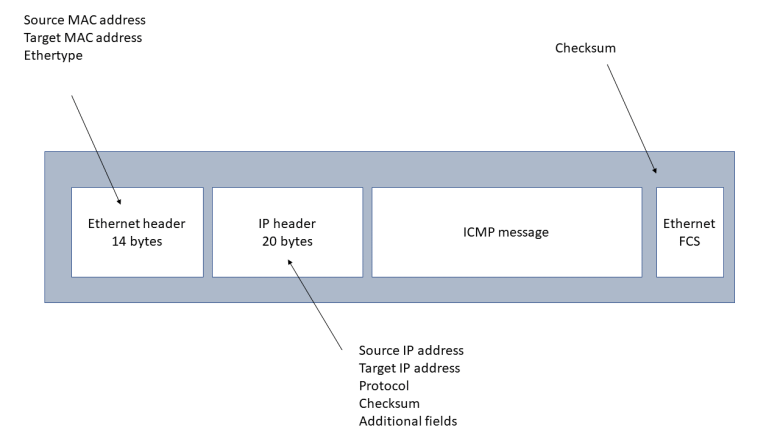
The first byte (0x45) of the IP header is in fact a combination of two fields. The first part (0x4) is the IP protocol version. The value 0x4 indicates IPv4, which is more and more replaced by IPv6. The second nibble (0x5) is the length of the header in units of 32 bit words, i.e. 20 bytes in this case.

The next byte (0x00 in our case) is called type of service and not used in our example. This field has been redefined several times in the history of the IP protocol but never been widely used – see the short article on Wikipedia for a summary.

The two bytes after the type of service are the total length of the packet, and are followed by two bytes called identification that are related to fragmentation that we will discuss further below. The same applies to
the next two bytes (0x4000 in hexadecimal notation or 0100000000000000 in binary notation).

The following two 8-bit fields are called time to live and the protocol. The time to live (TTL), 0x40 or 64 decimal in our case, specifies the time a packet will survive while being transmitted through the internet network. Whenever an IP packet is routed by a host in the network, the field will be reduced by one. When the value of the field reaches zero, the packet will be dropped. The idea of this is to avoid that a packet which cannot be delivered to its final destination circulates in the network forever. We will learn more about the process of routing in one of the following posts in this series.

The protocol field (0x1 in our case) is the equivalent of the ethertype in the Ethernet header. It indicates which protocol the payload belongs to. The valid values are specified in RFC790. Looking up the value 0x1 there, we find that it stands for ICMP as expected.

After the following two bytes which are the header checksum, we find the source address and destination address. Both addresses are encoded as 32 bit values, to be read as a sequence of four 8 bit values. The source address, for instance, is

c0 a8 b2 1b

If we translate each byte into a decimal value, this becomes

192 168 178 27

which corresponds to the usual notation 192.168.178.27 of the IP address of the PC on which the packet was generated. Similarly, the target address is 192.168.178.1.

In our case, the IP header is 20 bytes long, with the target address being the last field. The general layout allows for some additional options to be added to the header which we will not discuss here. Instead, we will now look at a more subtle point of the protocol – fragmentation.

Fragmentation

What is the underlying problem that fragmentation tries to solve? When looking at how the Ethernet protocol works, we have seen that the basic idea is to enable several stations to share a common medium. This only works because each station occupies the medium for a limited time, i.e. because an Ethernet frame has a limited size. Traditionally, an Ethernet frame is not allowed to be longer than 1518 bytes, where 18 bytes are reserved for the header and the checksum. Thus, the actual payload that one frame can carry is limited to 1500 bytes.

This number is called the maximum tranmission unit (MTU) of the medium. Other media like PPP or WLAN have different MTUs, but the size of a packet is also limited there.

Now suppose that a host on the internet wishes to assemble an IP packet with a certain payload. If the payload is so small that the payload including the header fit into the MTU of all network segments that the packet has to cross until it reaches its final destination, there is no issue. If, however, the total size of the packet exceeds the smallest MTU of all the network segments that the packet will visit (called the path MTU), we need a way to split the packet into pieces.

This is exactly what fragmentation is doing. Fragmentation refers to the process of splitting an IP packet into smaller pieces that are then reassembled by the receiver. This process involves the fields in the IP header that we have not described so far – the identification field and the two bytes immediately following it which consist of a 3 bit flags field and a 13 bit fragment offset field.

When a host needs to fragment an IP packet, it will split the payload into pieces that are small enough to pass all segments without further fragmentation (the host will typically use ICMP to determine the path MTU to the destination as we will see below). Each fragment receives its own IP header, with all fragments sharing the same values for the source IP address, target IP address, identification and protocol. The flags field is used to indicate whether a given fragment is the last one or is followed by additional fragments, and the fragment offset field indicates where the fragment belongs to in the overall message.

When a host receives fragments, it will reassemble them, using again the four fields identification, source address, target address and protocol. It can use the fragment offset to see where the fragment at hand belongs in the overall message to be assembled and the flags field to see whether a given fragment is the last one – so that the processing of the message can start – or further fragments need to be waited for. Note that the host cannot assume that the fragments arrive in the correct order, as they might travel along different network paths.

Note that the flags field also contains a bit which, if set, instructs all hosts not to fragment this datagram. Thus if the datagram exceeds one of the MTUs, it will be dropped and the sender will be informed by a so specific ICMP message. This process can be used by a sender to determine the path MTU on the way to the destination and is called path MTU discovery.

Packets can be dropped, of course, for other reasons as well. IP is inherently not establishing any guarantees that a message arrives at the destination, there are no handshakes, connections or acknowledgements. This is the purpose of the higher layer protocols like TCP that we will look at in a later post.

So far, we have ignored one point. When a host assembles an IP packet, it needs to determine the physical network interface to use for the transmission and the Ethernet address of the destination. And what if the target host is not even part of the same network? These decisions are part of a process called routing that we will discuss in the next post in this series.

Networking basics – Ethernet

In the previous post in this series, we have looked at the layered architecture of a typical network stack. In this post, we will dive into the lowest layer of a typical TCP/IP implementation – the Ethernet protocol.

The term Ethernet originally refers to a set of standards initially developed in the seventies by Xerox and then standardized jointly with DEC and Intel (see for instance this link to the original specification of what became knowns as Ethernet II). These standards describe both the physical layer (PHY), i.e. physical media, encoding, voltage levels, timing and so forth, as well as the data link layer that specifies the layout of the messages and the handling of collisions.

To understand how Ethernet works, it is useful to look at a typical network topology used by the early versions of the Ethernet standard. In such a setup, several hosts would be connected to a common medium in a bus topology, as indicated in the diagram below.EthernetBusTopology

 
Here, a shared medium – initially a coaxial cable – was used to transmit messages, indicated by the thick horizontal line in the diagram. Each station in the network is connected to this cable. When a station wants to transmit a message, it translates this message into a sequence of bits (Ethernet is inherently a serial protocol), checks that no other message is currently in transit and forces a corresponding voltage pattern onto the medium. Any other station can sense that voltage pattern and translate the message back.

Each station in the network is identified by a unique address. This address is an 48 bit number called the MAC address. When a station detects an Ethernet message (called a frame) on the shared medium, it extracts the target address from that frame and compares it to its own MAC address. If they do not match, the frame is ignored (there are a few exceptions to this rule, as there are broadcast addresses and a device can be operated in promiscuity mode in which it will pick up all frames regardless of their target address).

There is one problem, though. What happens if several stations want to transmit messages at the same time? If that happens, the signals overlap and the transmission is disturbed. This is called a collision. Part of the Ethernet protocol is a mechanism called CSMA/CD (carrier sense multiple access with collision detection) that specifies how these situations are detected and handled. Essentially, the idea is that a a station that detects a collision will wait for a certain random time and simply retry. If that fails again, it will again wait, using a different value for the wait time. After a certain number of failed attempts, the transmission will be aborted.

This mechanisms works a bit like a conference call. As you cannot see the other participants, it is very hard to tell whether someone wants to speak. So you first wait for some time, and if nobody else has started to talk, you start. If there is still a collision, both speakers will back off and wait for some time, hoping that their next attempt will be successful. Given the random wait times, it is rather likely that using this procedure, one of the speakers will be able to start talking after a few attempts.

This is nice and worked well for smaller networks, but has certain disadvantages when striving for larget networks with higher transfer rates. First, collision resolution consumes time and slows down the traffic significantly if too many collisions occur. Second, communication in this topology is half-duplex: every station can either transmit or receive, but not both at the same time. Both issues are addressed in more modern networks where a switch-based topology is used.

A switch or bridge is an Ethernet device that can connect several physical network segments. A switch has several ports to which network segments are connected. A switch knows (in fact, it learns that information over time) which host is connected to which port. When an Ethernet frame arrives at one of the ports, the switch uses that information to determine the port to which the frame needs to be directed and forwards the frame to this port.

EthernetSwitchedTopology

In such a topology, collisions can be entirely avoided once the switch has learned which device is behind which port. Each station is connected to the switch using a twisted pair cable and can talk to the switch in full duplex mode (if the connection allows for it), i.e. receive and transmit at the same point in time.  Most switches have the ability to buffer a certain amount of data to effectively serialize the communication at the individual ports, so that collisions can be avoided even if two frames for the same destination port arrive at the switch simultaneously. This sort of setup is more expensive due to the additional costs for the switches, but has become the standard topology even in small home networks.

Having looked at the physical realization of an Ethernet network, let us now try to observe this in action.  For these tests, I have used my home PC running Ubuntu Linux 16.04 which is connected to a home network via an Ethernet adapter.  This adapter is known to the operating system as enp4s0 (on older Ubuntu versions, this would be eth0).

First, let us collect some information about the local network setup using the tool ifconfig.

$ ifconfig enp4s0
enp4s0    Link encap:Ethernet  HWaddr 1c:6f:65:c0:c9:85  
          inet addr:192.168.178.27  Bcast:192.168.178.255  Mask:255.255.255.0
          inet6 addr: fe80::dd59:ad15:4f8e:6a87/64 Scope:Link
          UP BROADCAST RUNNING MULTICAST  MTU:1500  Metric:1
          RX packets:48431 errors:0 dropped:0 overruns:0 frame:0
          TX packets:37871 errors:0 dropped:0 overruns:0 carrier:0
          collisions:0 txqueuelen:1000 
          RX bytes:46537519 (46.5 MB)  TX bytes:7483354 (7.4 MB)

Here we see that our network device enps4s0 is an Ethernet device with the MAC address 1c:6f:65:c0:c9:85. Here the 48 bit MAC address is printed as a sequence of 6 bytes, separated by colons.

Now open a terminal, become root and enter the following command:

tcpdump -i enp4s0 -xxx

This will instruct tcpdump to dump packages going over enp4s0, printing all details including the Ethernet header (-xxx). On another terminal, execute

ping 192.168.178.1

Then tcpdump will produce the following output (plus a lot of other stuff, depending on what you currently run in parallel):

21:28:18.410185 IP your.host > your.router: ICMP echo request, id 6182, seq 1, length 64
0x0000: 0896 d775 7e80 1c6f 65c0 c985 0800 4500
0x0010: 0054 e6a3 4000 4001 6e97 c0a8 b21b c0a8
0x0020: b201 0800 4135 1826 0001 d233 de5a 0000
0x0030: 0000 2942 0600 0000 0000 1011 1213 1415
0x0040: 1617 1819 1a1b 1c1d 1e1f 2021 2223 2425
0x0050: 2627 2829 2a2b 2c2d 2e2f 3031 3233 3435
0x0060: 3637
21:28:18.412823 IP your.router > your.host: ICMP echo reply, id 6182, seq 1, length 64
0x0000: 1c6f 65c0 c985 0896 d775 7e80 0800 4500
0x0010: 0054 0b2c 0000 4001 8a0f c0a8 b201 c0a8
0x0020: b21b 0000 4935 1826 0001 d233 de5a 0000
0x0030: 0000 2942 0600 0000 0000 1011 1213 1415
0x0040: 1617 1819 1a1b 1c1d 1e1f 2021 2223 2425
0x0050: 2627 2829 2a2b 2c2d 2e2f 3031 3233 3435
0x0060: 3637

Let us examine this output in detail. Each packet printed by tcpdump is an Ethernet frame. Every frame starts with an Ethernet specific part called the Ethernet header followed by a part determined by the higher layers of the protocol stack that we will not discuss in this but in later posts.

The first Ethernet frame starts with the destination MAC address 08:96:d7:75:7e:80 which in this case is the MAC address of my router (you can figure out the MAC address of your router using the `arp` command).

The next six bytes in the frame contain the source MAC address 1c:6f:65:c0:c9:85, i.e. the MAC address of my network card in this case. Note that this matches the output of `ifconfig` displayed above.

The next two bytes of the Ethernet frame are still part of the header and are called the ethertype. This field holds a number that specifies the higher layer protocol to which the data in the Ethernet frame refers. This field is not used by the Ethernet protocol itself, but is relevant for an operating system as it determines to which protocol stack the content of the Ethernet frame is routed for further processing. In our case, the ethertype is 0x800, indicating that this is an IP request.

The next bytes starting with the value 0x45 form the data part of the Ethernet frame and contain the actual payload.

In addition to the data displayed by tcpdump, there are additional bytes at the start and end of each Ethernet frame that are handled by the network card and usually not visible to applications. Preceding the Ethernet header, there is a so called preamble which is a fixed 56 bit pattern designed to allow the stations to synchronize their clock. The preamble is followed by an 8-bit pattern called the start frame delimiter (SDF), which is again a fixed value indicating the start of the actual frame (in some sources, the SFD is considered to be part of the preamble). These bits are then followed by the fields described above:

  • Destination MAC address
  • Source MAC address
  • Ethertype
  • Data

Finally, the Ethernet frame ends with a checksum called Frame check sequence which is used to detect transmission errors.

This simple structure of an Ethernet frame is virtually unchanged compared to the original Ethernet II specification. However, over time, some extensions and protocol variations have been defined. The most notable one is VLAN tagging according to the IEEE 802.1Q standard.

A VLAN or virtual LAN is a technology to split a single Ethernet network into logically separated areas. One way to do this is to program switches in such a way that they assign stations and the corresponding ports to different virtual LANs and allow traffic to flow only within each VLAN. However, this simple implementation fails if the network spans more than one switch. To support these cases as well, an Ethernet frame can contain an optional field – the VLAN tag – that contains the ID of the virtual LAN in which the frame is supposed to be distributed. This tag is placed right after the ethertype. To indicate its presence, the dummy ethertype 0x8100 is used, followed by the VLAN tag and the actual ethertype.

This concludes our short introduction to the Ethernet protocol. In the next post, we will discuss the network layer and the IP protocol before we then move on to ARP and routing.

References


Networking basics – the layered networking model

Recently, I picked up an old project of mine – implementing a Unix like operating kernel from scratch. I will post more on this later, but one of the first things I stumbled across when browsing my old code and my old documentation was the networking stack. I used this as an opportunity to refresh my own understanding of networking basics, and reckoned it might help others to post my findings here. So I decided to write a short series of posts on the basics of networking – ethernet, ARP, IP, TCP/UDP and all that stuff.

Before we start to get into details on the different networking technologies, let me first explain the idea of a layered networking architecture.

Ultimately, networking is about physical media (copper cables, for instance) connecting physical machines. Each of these machines will be connected to the network using a network adapter. These adapters will write messages into the network, i.e. create a certain sequence of electrical signals on the medium, and read other messages coming from the network.

However, the magic of a modern networking architecture is that the same physical network can be used to connect different machines with different operating systems using different networking protocols. When you use your web browser to connect to some page on the web – this one for instance – your web browser will use a protocol called HTTP(S) for that purpose. From the web browsers point of view, this appears to be a direct connection to the web server. The underlying physical network can be quite different – it can be a combination of Ethernet or WLAN to connect your PC to a router, some technology specific to your ISP or even a mobile network. The beauty of that is that the browser does not have to care. As often in computer science, this becomes possible by an abstract model organizing networking capabilities into layers.

Several models for this layering exist, like the OSI model and the TCP/IP layered model defined in RFC1122. For the sake of simplicity, let us use the four-layer TCP/IP model as an example.


TCPIPLayers


The lowest layer in this model is called the link layer. Roughly speaking, this layer is the layer which is responsible for the actual physical connection between hosts. This covers things like the physical media connecting the machines and the mechanisms used to avoid collisions on the media, but also the addressing of network interfaces on this level.

One of the most commonly used link layer protocols is the Ethernet protocol. When the Ethernet protocol is used, hosts in the network are addressed using the so-called MAC address which uniquely identifies a network card within the network. In the Ethernet protocol (and probably in most other protocols), the data is transmitted in small units called packets or frames. Each packet contains a header with some control data like source and destination, the actual data and maybe a checksum and some end-of-data marker.

Now Ethernet is the most common, but by far not the only available link layer protocol. Another protocol which was quite popular at some point at the end of the last century is the Token Ring protocol, and in modern networks, a part of the path between two stations could be bridged by a provider specific technology or a mobile network. So we need a way to make hosts talk to each other which are not necessarily connected via a direct Ethernet link.

The approach taken by the layered TCP/IP model to this is as follows. Suppose you have – as in the diagram below – two sets of machines that are organized in networks. On the left hand side, we see an Ethernet network with three hosts that can talk to each other using Ethernet. On the right hand side, there is a smaller network that consists of two hosts, also connected with each other via Ethernet (this picture is a bit misleading, as in a real modern network, the topology would be different, but let us ignore this for a moment).

NetworksAndGatewaysBoth networks are connected by a third network, indicated by the dashed line. This network can use any other link layer technology. Each network contains a dedicated host called the gateway that connects the network to this third network.

Now suppose host A wants to send a network message to host B. Then, instead of directly using the link layer protocol in its network, i.e. Ethernet, it composes a network message according to a protocol that is in the second layer of the TCP/IP networking model, called the Internet layer which uses the IP protocol. Similar to an Ethernet packet, this IP packet contains again a header with target and source address, the actual data and a checksum.

Then host A takes this message, puts that into an Ethernet packet and sends it to the gateway. The gateway will now extract the IP message from the Ethernet packet, put it into a message specific to the networking connecting the two gateways and transmit this message.

When the message arrives at the gateway on the right hand side, this gateway will again extract the IP message, put it into an Ethernet message and send this via Ethernet to host B. So eventually, the unchanged IP message will reach host B, after traveling through several networks, piggybacked on messages specific to the used network protocols. However, for applications running on host A and B, all this is irrelevant – they will only get to see IP messages and do not have to care about the details and layer below.

In this way, the internet connects many different networks using various different technologies – you can access hosts on the internet from your mobile device using mobile link layer protocols, and still communicate with a host in a traditional data center using Ethernet or something else. In this sense, the internet is a network of networks, powered by the layer model.

But we are not yet done. The IP layer is nice – it allows us to send messages across the internet to other hosts, using the addresses specific to the IP layer (yes, this is the IP address). But it does, for instance, not yet guarantee that the message ever arrives, nor does it provide a way to distinguish between different communication end points (aka ports) on one host.

These items are the concern of the next layer, the transport layer. The best known example of a transport layer protocol is TCP. On top of IP, TCP offers features like stream oriented processing, re-transmission of lost messages and ports as additional address components. For an application using TCP, a TCP connection appears a bit like a file into which bytes can be written and out of which bytes can be read, in a well defined order and with guaranteed delivery.

Finally, the last layer is the application layer. Common application layer protocols are HTTP (the basis of the world wide web), FTP (the file transfer protocol), or SMTP (the mail transport protocol).

The transitions between the different layers work very much like the transition between the internet layer and the link layer. For instance, if an application uses TCP to send a message, the operating system will take the message (not exactly true, as TCP is byte oriented and not message oriented, but let us gracefully ignore this), add a TCP header, an IP header and finally an Ethernet header, and ask the network card to transmit the message on the Ethernet network. When the message is received by the target host, the operating system of that host strips off the various headers one by one and finally obtains the original data sent by the first host.

The part of the operating system responsible for this mechanism is naturally itself organized in layers  – there could for instance be an IP layer that receives data from higher layers without having to care whether the data represents a TCP message or a UDP message. This layer then adds an IP header and forwards the resulting message to another layer responsible for operating the Ethernet network device and so forth. Due to this layered architecture stacking different components on top of each other, the part of the operating system handling networking is often called the networking stack. The Linux kernel, for instance, is loosely organized in this way (see for instance this article).

This completes our short overview of the networking stack. In the next few posts, we will look at each layer one by one, getting our hands dirty again, i.e. we will create and inspect actual network messages and see the entire stack in action.


More on Paperspace Gradient

Its been a few days since I started to play with Paperspace, and I have come across a couple of interesting features that the platform has – enough for a second post on this topic.

First, GIT integration. Recall that the usual process is to zip the current working directory and submit the resulting file along with the job, the ZIP file is then unzipped in the container in which the job is running and the contents of the ZIP file constitute the working directory. However, if you want to run code that requires, for instance, custom libraries, it is much easier to instruct Paperspace to get the contents of the working directory from GitHub. You can do that by supplying a GIT URL using the --workspace switch. The example below, for instance, instructs Paperspace to pull my code for an RBM from GitHub and to run it as a job.

#!/bin/sh
#
# Run the RBM as a job on Paperspace. Assume that you have the paperspace NodeJS
# CLI and have done a paperspace login before to store your credentials
#
#
~/node_modules/.bin/paperspace jobs create  \
        --workspace "git+https://github.com/christianb93/MachineLearning" \
        --command "export MPLBACKEND=AGG ; python3 RBM.py \
        --N=28 --data=MNIST \
        --save=1 \
        --tmpdir=/artifacts \
        --hidden=128 \
        --pattern=256 --batch_size=128 \
        --epochs=40000 \
        --run_samples=1 \
        --sample_size=6,6 \
        --beta=1.0 --sample=200000 \
        --algorithm=PCDTF --precision=32" \
        --machineType K80 \
        --container "paperspace/tensorflow-python" \
        --project "MachineLearning"

Be careful, the spelling of the URL must be exactly like this to be recognized as a GIT URL, i.e. “git+https” followed by the hostname without the “www”, if you use http instead of https or http://www.github.com instead of github.com, the job will fail (the documentation at this point could be better, and I have even had to look at the source code of the CLI to figure out the syntax). This is a nice feature, using that along with the job logs, I can easily reconstruct which version of the code has actually been executed, and it supports working in a team that is sharing GitHub repositories well.

Quite recently, Paperspace did apparently also add the option to use persistent storage in jobs to store data across job runs (see this announcement). Theoretically, the storage should be shared between notebooks and jobs in the same region, but as I have not yet found out how to start a notebook in a specific region, I could not try this out.

Another feature that I liked is that the container that you specify can actually be any container from the Docker Hub, for instance ubuntu. The only restriction is that Paperspace seems to overwrite the entrypoint in any case and will try to run bashinside the container to finally execute the command that you provide, so containers that do not have a bash in the standard execution path will not work. Still, you could use this to prepare your own containers, maybe with pre-installed data sets or libraries, and ask Paperspace to run them.

Finally, for those of us who are Python addicts, there is also a Python API for submitting and managing jobs in Paperspace. Actually, this API offers you two ways to run a Python script on Paperspace. First, you can import the paperspace package into your script and then, inside the script, do a paperspace.run(), as in the following example.

import paperspace
paperspace.run()
print('This will only be running on Paperspace')

What will happen behind the scenes is that the paperspace module takes your code, removes any occurrences of the paperspace package itself, puts the code into a temporary file and submits that as a job to Paperspace. You can then work with that job as with any other job, like monitoring it on the console or via the CLI.

That is nice and easy, but not everyone likes to hardcode the execution environment into the code. Fortunately, you can also simply import the paperspace package and use it to submit an arbitrary job, much like the NodeJs based CLI can do it. The code below demonstrates how to create a job using the Python API and download the output automatically (this script can also be found on GitHub).

import paperspace.jobs
from paperspace.login import apikey
import paperspace.config

import requests


#
# Define parameters
#
params = {}
# 
# We want to use GIT, so we use the parameter workspaceFileName
# instead of workspace
#
params['workspaceFileName'] = "git+https://github.com/christianb93/MachineLearning"
params['machineType'] = "K80"
params['command'] = "export MPLBACKEND=AGG ; python3 RBM.py \
                --N=28 --data=MNIST \
                --save=1 \
                --tmpdir=/artifacts \
                --hidden=128 \
                --pattern=256 --batch_size=128 \
                --epochs=40000 \
                --run_samples=1 \
                --sample_size=6,6 \
                --beta=1.0 --sample=200000 \
                --algorithm=PCDTF --precision=32"
params['container'] = 'paperspace/tensorflow-python'
params['project'] = "MachineLearning"
params['dest'] = "/tmp"

#
# Get API key
#
apiKey = apikey()
print("Using API key ", apiKey)
#
# Create the job. We do NOT use the create method as it cannot
# handle the GIT feature, but assemble the request ourselves
#
http_method = 'POST'
path = '/' + 'jobs' + '/' + 'createJob'


r = requests.request(http_method, paperspace.config.CONFIG_HOST + path,
                             headers={'x-api-key': apiKey},
                             params=params, files={})
job = r.json()
    
if 'id' not in job:
    print("Error, could not get jobId")
    print(job)
    exit(1)

jobId = job['id']
print("Started job with jobId ", jobId)
params['jobId']  = jobId

#
# Now poll until the job is complete

if job['state'] == 'Pending':
    print('Waiting for job to run...')
    job = paperspace.jobs.waitfor({'jobId': jobId, 'state': 'Running'})

print("Job is now running")
print("Use the following command to observe its logs: ~/node_modules/.bin/paperspace jobs logs --jobId ", jobId, "--tail")

job = paperspace.jobs.waitfor({'jobId': jobId, 'state': 'Stopped'})
print("Job is complete: ", job)

#
# Finally get artifacts
#
print("Downloading artifacts to directory ", params['dest'])
paperspace.jobs.artifactsGet(params)

There are some additional features that the Python API seems to have that I have not yet tried out. First, you can apparently specify an init script that will be run before the command that you provide (though the use of that is limited, as you could put this into your command as well). Second, and more important, you can provide a requirements file according to the pip standard to ask Paperspace to install any libraries that are not available in the container before running your command.

Overall, my impression is that these APIs make it comparatively easy to work with jobs on Paperspace. You can submit jobs, monitor them and get their outputs, and you enjoy the benefit that you are only billed for the actual duration of the job. So if you are interested in a job based execution environment for your Machine Learning models, it is definitely worth a try, even though it takes some time to get familiar with the environment.