
In the last post, we have looked at the Deutsch-Jozsa algorithm that is considered to be the first example of a quantum algorithm that is structurally more efficient than any classical algorithm can probably be. However, the problem solved by the algorithm is rather special. This does, of course, raise the question whether a similar speed-up can be achieved for problems that are more relevant to practical applications.
In this post, we will discuss an algorithm of this type – Grover’s algorithm. Even though the speed-up provided by this algorithm is rather limited (which is of a certain theoretical interest in its own right), the algorithm is interesting due to its very general nature. Roughly speaking, the algorithm is concerned with an unstructured search. We are given a set of N = 2n elements, labeled by the numbers 0 to 2n-1, exactly one of which having a property denoted by P. We can model this property as a binary valued function P on the set 
Grover’s algorithm
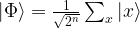
Grover’s algorithm presented in [1] proceeds as follows to locate this element. First, we again apply the Hadamard-Walsh operator W to the state 
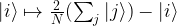
- Apply a conditional phase shift S, i.e. apply the unique unitary transformation that maps
to
.
- Apply the unitary transformation D called diffusion that we will describe below
Finally, after a defined number of outcomes, we perform a measurement which will collaps the system into one of the states
Before we can proceed, we need to define the matrix D. This matrix is 

Consequently, we see that

where 

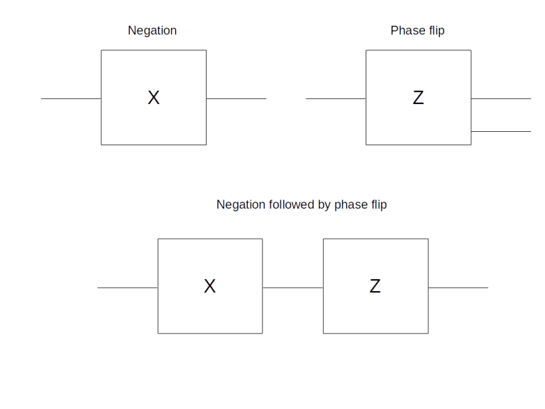
For the sake of completeness, let us also briefly discuss the first transformation employed by the algorithm, the conditional phase shift. We have already seen a similar transformation while studying the Deutsch-Jozsa algorithm. In fact, we have shown in the respective blog post that the circuit displayed below (with the notation slightly changed)
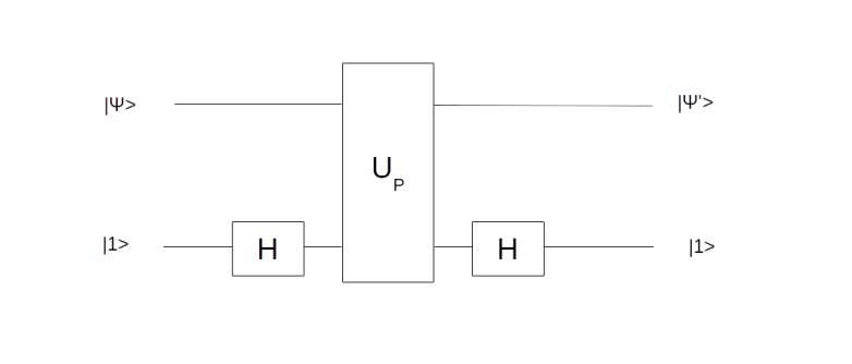
performs the required operation

Let us now see how why Grover’s algorithm works. Instead of going through the careful analysis in [1], we will use bar charts to visualize the quantum states (exploiting that all involved matrices are actually real valued).
It is not difficult to simulate the transformation in a simple Python notebook, at least for small values of N. This script performs several iterations of the algorithm and prints the result. The diagrams below show the outcome of this test.
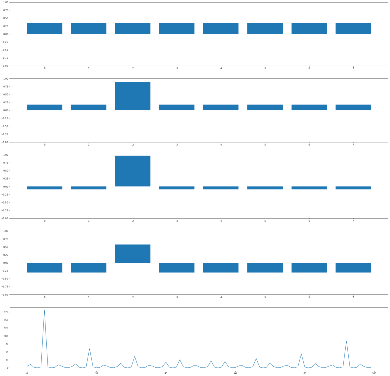
Let us go through the diagrams one by one. The first diagram shows the initial state of the algorithm. I have used 3 qubits, i.e. n = 3 and N = 8. The initial state, after applying the Hadamard-Walsh transform to the zero state, is displayed in the first line. As expected, all amplitudes are equal to 1 over the square root of eight, which is approximately 0.35, i.e. we have a balanced superposition of all states.
We now apply one iteration of the algorithm. First, we apply the conditional phase flip. The element we are looking for is in this case located at x = 2. Thus, the phase flip will leave all basis vectors unchanged except for 
Thus, what really happens in this case is an amplitude amplification – we increase the amplitude of one component of the superposition while decreasing all the others.
The next few lines show the result of repeating these two steps. We see that after the second iteration, almost all of the amplitude is concentrated on the vector
It is interesting to see that when we perform one more iteration, the difference between the amplitude of the solution and the amplitudes of all other components decreases again. Thus the correct choice for the number of iterations is critical to make the algorithm work. In the last line, we have plotted the difference between the amplitude of 
Generalizations and amplitude amplification
In a later paper ([3]), Grover describes a more general setup which is helpful to understand the basic reason why the algorithm works – the amplitude amplification. In this paper, Grover argues that given any unitary transformation U and a target state (in our case, the state representing the solution to the search problem), the probability to meet the target state by applying U to a given initial state can be amplified by a sequence of operations very much to the one considered above. We will not go into details, but present a graphical representation of the algorithm.
So suppose that we are given an n-qubit quantum system and two basis vectors – the vector t representing the target state and an initial state s. In addition, assume we are given a unitary transformation U. The goal is to reach t from s by subsequently applying U itself and a small number of additional gates.
Grover considers the two-dimensional subspace spanned by the vectors s and U-1t. If, within this subspace, we ever manage to reach U-1t, then of course one more application of U will move us into the desired target state.
Now let us consider the transformation
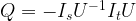
where Ix denotes a conditional phase shift that flips the phase on the vector
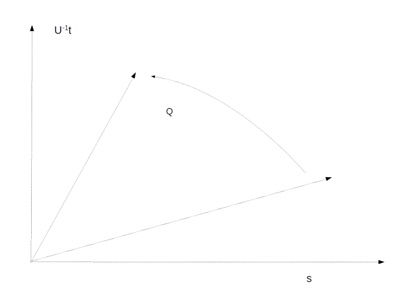
He then proceeds to show that for sufficiently small values of the matrix element Uts, the action of Q on this subspace can approximately be described as a rotation by the angle 

Thus if we can make the first coefficient very small, i.e. if 

Let us link this description to the version of the Grover algorithm discussed above. In this version, the initial state s is the state 

This can be written as

Regrouping this and using the relation D = -W I0 W, we see that this is the same as

Thus the algorithm can equally well be described as applying W once to obtain a balanced superposition and then applying the sequence DS n times, which is the formulation of the algorithm used above. As 
Applications
Grover’s algorithm is highly relevant for theoretical reasons – it applies to a very generic problem and (see the discussions in [1] and [2]) is optimal, in the sense that it provides a quadratic speedup compared to the best classical algorithm that requires O(N) operations, and that this cannot be improved further. Thus Grover’s algorithm provides an interesting example for a problem where a quantum algorithm delivers a significant speedup, but no exponential speedup as we will see it later for Shor’s algorithm.
However, as discussed in detail in section 9.6 of [4], the relevance of the algorithm for practical applications is limited. First, the algorithm applies to an unstructured search, i.e. a search over unstructured data. In most practical applications, we deal with databases that have some sort of structure, and then more efficient search algorithms are known. Second, we have seen that the algorithm requires 
Examples of such problems are brute forces searches as they appear in some crypto-systems. Suppose for instance we are trying to break a message that is encrypted with a symmetric key K, and suppose that we know the first few characters of the original text. We could then try to use an unstructured search over the space of all keys to find a key which matches at least the few characters that we know.
In [5], a more detailed analysis of the complexity in terms of qubits and gates that a quantum computer would have to attack AES-256 is made, arriving at a size of a few thousand logical quantum bits. Given the current ambition level, this does not appear to be completely out of reach. It does, however, not render AES completely unsecure. In fact, as Grover’s algorithm essentially results in a quadratic speedup, a code with a key length of n bits in a pre-quantum world is essentially as secure as the same code with a key length of 2n in a post-quantum world, i.e. roughly speaking, doubling the key length compensates the advantage of quantum computing in this case. This is the reason why the NIST report on post-quantum cryptography still classifies AES as inherently secure assuming increased key sizes.
In addition, the feasibility of a quantum algorithm is not only determined by the number of qubits required, but also by other factors like the depth, i.e. the number of operations required, and the number of quantum gates – and for AES, the estimates in [5] are significant, for instance a depth of more than 2145 for AES-256, which is roughly 1043. Even if we assume a switching time of only 10-12 seconds, we still would require astronomical 1031 seconds, i.e. in the order of 1023 years, to run the algorithm.
Even a much less sophisticated analysis nicely demonstrates the problem behind these numbers – the number of iterations required. Suppose we are dealing with a key length of n bits. Then we know that the algorithm requires

iterations. Taking the decimal logarithm, we see that this is in the order of 100.15*n. Thus, for n = 256, we need in the order of 1038 iterations – a number that makes it obvious that AES-256 can still be considered secure for all practical purposes.
So overall, there is no reason to be overly concerned about serious attacks to AES with sufficiently large keys in the near future. For asymmetric keys, however, we will soon see that the situation is completely different – algorithms like RSA or Elliptic curve cryptography are once and for all broken as soon as large-scale usable quantum computer become reality. This is a consequence of Shor’s algorithm that we will study soon. But first, we need some more preliminaries that we will discuss in the next post, namely quantum Fourier transforms.
References
1. L.K. Grover, A fast quantum mechanical algorithm for database search, Proceedings, 28th Annual ACM Symposium on the Theory of Computing (STOC), May 1996, pages 212-219, available as arXiv:quant-ph/9605043v3
[2] M. Boyer, G. Brassard, P. Høyer, A. Tapp, Tight bounds on quantum searching, arXiv:quant-ph/9605034
3. L.K. Grover, A framework for fast quantum mechanical algorithms, arXiv:quant-ph/9711043
4. E. Rieffel, W. Polak, Quantum computing – a gentle introduction, MIT Press
5. M. Grassl, B. Langenberg, M. Roetteler, R. Steinwandt, Applying Grover’s algorithm to AES: quantum resource estimates, arXiv:1512.04965


 and consider the function
 with
with  and
and  to
to  , where
  is the bitwise exlusive or, we obtain an invertible function (as
  ), and we can recover our old function
  if we let
  .
.  , with the natural numbers between 0 and 2l-1 and these numbers in turn with elements of the standard basis – the bit string
  for instance would correspond to the element of the standard basis that we denote by
  . Thus, the function described above defines a permutation of the elements of the standard basis. Consequently, by the rules of linear algebra, there is exactly one unitary transformation Uf with the property that (with that identification)
 . First, we can write this as

 appears exactly once, where x ranges from 0 to 2n-1. Consequently, we see that
 and the identity to the remaining m qubits. Thus, our initial state will be
 obtained above, we easily see that applying this transformation to our initial state yields the state
 and
and  by a set of quantum gates
 , i.e. to the basis of our Hilbert space, then applying that measurement would yield a state
 . Thus to retrieve the value of f(x) for a given value of x, we would have a rather small probability to be successful with only one pass of the algorithm.
 where x is a n-bit number and y is 0 or 1. We again obtain an initial state
 . The algorithm then proceeds by applying Uf resulting in the state


 . As clearly

 , depending on the sign of f. Thus our measurement will give us one with certainty, as our state is simply a scalar multiple of
  , say to

 .
.  from the
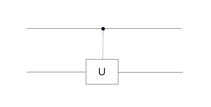
  with only one application of Uf. It uses an ancilla qubit that is initialized in the state
  . The graphical representation is as follows.
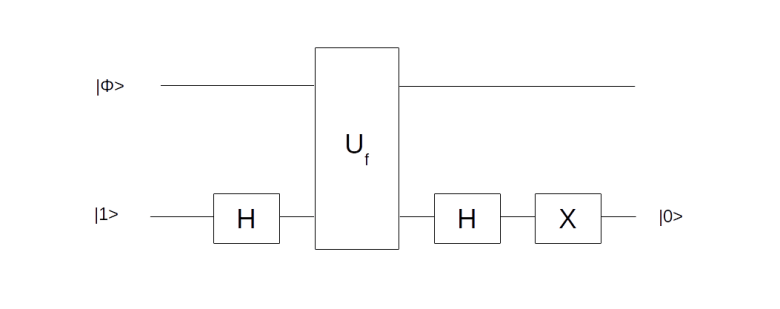

 to itself and
  to itself. If, however, f(x) is one, it maps


 , a unitary transformation is of course given by a unitary 2×2 matrix.
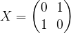
 and is therefore sometimes called the bit-flip or negation. Its eigenvalues are 1 and -1, with a pair of orthogonal and normed eigenvectors given by


 and
and  , and, as
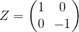
  , vice versa. Similarly, the phase operator
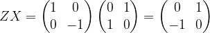
 for this. In this basis, the CNOT gate is given by the following 4 x 4 matrix:
 and
and  to itself and swaps the vectors
  and
and  . Thus, expressed in terms of bits, it negates the second bit if the first bit is ON and keeps the second bit as it is if the first bit is OFF. Thus, the first bit can be thought of as a control bit that controls whether the second bit – the target bit – is toggled or not, and this is where the name comes from, CNOT being the abbreviation for “controlled NOT”. Graphically, the CNOT gate is represented by a small circle on the control bit and an encircled plus sign on the target bit (this is the convention used in
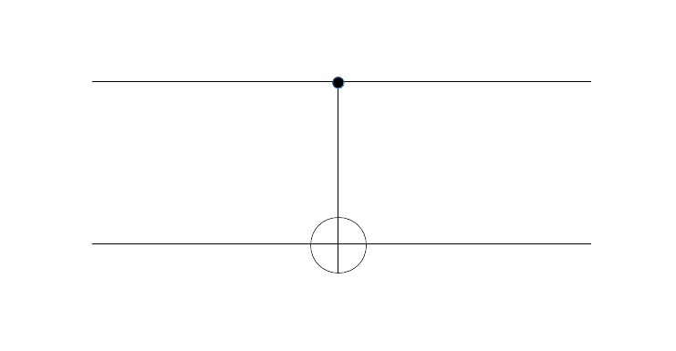
 . This state can as well be written as

 . We read the circuit from the left to the right and the top to the bottom. Thus, the first part of the circuit acts with H on the first qubit and with the identity on the second qubit. It therefore maps the state

 to
to  . Thus the entire circuit maps the vector
 to
to  , and it is well known that any such function can be expressed as a combination of gates from a small set of standard gates called universal gates. In fact, it is even true that one gate is sufficient – the NAND gate. It is natural to ask whether the same is true for quantum gates. More precisely, can we find a finite set of unitary transformations such that any n-qubit unitary transformation can be composed from them using a few standard operations like the tensor product?
 phase gate.