Quantum simulation

In his famous lecture Simulating Physics with computers, Nobel laureate Richard Feynman argued that non-trivial quantum systems cannot efficiently be simulated on a classical computer, but on a quantum computer – a claim which is widely considered to be one of the cornerstones in the development of quantum computing. Time to ask whether a universal quantum computer can deliver on that promise.

At the first glance, this seems to be obvious. Of course, there is one restriction – similar to classical computing, the resources of a quantum computer are finite, se we can only hope to be successful if we can at least approximately reduce the Hilbert space of the original problem to a finite dimensional space. But once this hurdle is taken, everything else looks easy. The time evolution of the system is governed by its Hamiltonian H – over a period of time t, the evolution of the system is described by the unitary operator

This is a unitary operator, so given a universal set of quantum gates, we should – at least approximately – be able to implement this unitary evolution as a sequence of quantum gates. And we are able to store a state in a Hilbert space of dimension 2^N in N qubits, in contrast to the exponential number of classical bits that we would need. So what is the problem?

The problem is hidden in the complexity to construct an arbitrary unitary operator from a finite set of quantum gates. Suppose we are considering a quantum system with a finite number of qubits N so that a unitary operator is described by an 2^N x 2^N matrix. As argued in [1], if we assemble unitary operators from a set of universal gates, we need in the order of 2^2N steps, as this number of parameters is required to specify an arbitrary (binary) matrix of size N. Thus we have mastered the memory bottleneck only to run into a time bottleneck, as the number of steps still grows exponentially with the dimension of the Hilbert space.

In addition, figuring out how to build up the unitary matrix from the given set of universal gates – a task typically accomplished with a classical computer – can still be extremely difficult and scale exponentially with N. So it seems that we are fighting a lost battle (see also section 4.5.4 of [2] for an argument why building general unitary matrices from an elementary set of gates is hard).

Fortunately, this is only true if we insist on simulating any conceivable unitary matrix. In practice, however, most Hamiltonians are much simpler and built from local interactions – and this turns out to be the key to efficiency.

As an example to illustrate this point, let us consider a typical system of interest – a lattice in space that has a particle of spin 1/2 attached to each of its vertices. Suppose further that any particle only interacts with adjacent particles. Then, in the easiest case of constant coupling, the Hamiltonian of this system can be written as

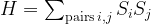
with spin operators S_i. The number of terms in the sum is proportional to N as we only allow pairs of adjacent spins to interact – actually it is roughly equal to 2N (each spin site pairs up with four other spins, and we need to divide by two as we double count – and there will be slight deviations from this rule depending on the boundary conditions). At every spin site, we have a two-dimensional Hilbert space describing that spin. If two sites i and j are adjacent, the operator S_iS_j acts on the tensor product of the Hilbert spaces attached to the involved sites, i.e. on a subspace of dimension four of the overall Hilbert space. The crucial point is that even though the dimension of the overall Hilbert space is huge, each term in the Hamiltonian only acts on a rather small subspace.

Let us now consider more general Hamiltonians of this form. Specifically, let us assume that we can write our Hamiltonian as a sum

of l = 2N hermitian operators, where each H_s only acts on a subspace of dimension m_s. Let m be an upper bound on the m_s.

Of course, it is general not true that the exponential of H is the product of the exponentials of the H_i, unless the H_i commute. So

However, it turns out that this equality becomes approximately true for very small times t. In fact, the Trotter formula states that

Thus, to simulate the development of the system over a certain time t, we could proceed as follows.

• Choose a large number n
• Initialize the quantum computer in a state corresponding to the initial state
• Apply each of the l operators e^iH_st/n in turn
• Repeat this n times
• Measure to determine the result

Note that in the last step, we typically do not measure all the individual qubits, but instead we are interested in the value of an observable A and measure that observable. In general, we will have to repeat the entire simulation several times to determine the expectation value of the measurement outcome.

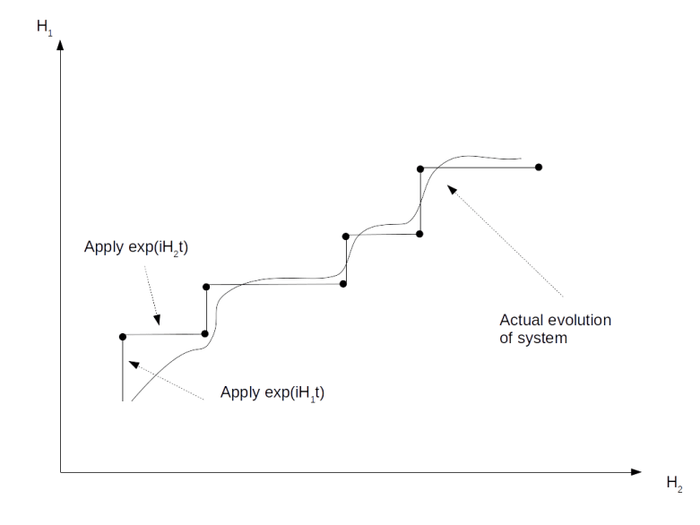
We can visualize the evolution of the quantum state under this process similar to the process of approximating a smooth curve by moving along the coordinate axis. If, for instance, l = 2, so that H = H₁ + H₂, we will periodically first apply e^iH₁t, then e^iH₂t and so forth. We can think of the two operators as coordinates, and then applying these operators corresponds to moving along the coordinate axis. If we move in sufficiently short intervals, we will at least approximately move along the smooth curve.

Now let us try to understand the complexity of this process. Each individual H_s acts on a space with dimension at most m. The important part is that if we enlarge the system – for instance by adding additional sites to a spin lattice – the number m is not substantially changed. Thus the unitary operator e^iH_st/n can be approximated by universal quantum gates in the order of m² steps, and the entire process takes in the order of nlm² steps. If l grows at most polynomially with N, as in our example of the spin lattice, the complexity therefore grows at most polynomially with N as well. In general, this will be exponential faster than on a classical computer.

The upshot of the discussion is that even though general unitary transformations are hard to approximate with a universal set of gates, local Hamiltonians – and therefore the Hamiltonians of a large and very rich class of interesting quantum systems – can be efficiently simulated by a universal quantum computer.

The method presented above (sometimes called the Trotter-based quantum simulation) is quite universal, but in some cases, special problems admit more specialized solutions that are also often termed as simulations. Suppose, for instance, we wanted to know the lowest energy eigenvalue of a quantum system. We could do this with our simulation approach – we start with an arbitrary state and simulate the system for some time, hoping that the system will settle in the ground state.

Obviously, this is not very efficient, and we might want to employ different methods. We have already seen that one possible approach to this is the variational quantum eigensolver treated in a previous post. However, there is also an approach related to the universal simulation described above. Basically, the idea described in [4] is to use quantum phase estimation to find the eigenvalues of U = e^iHt and hence of H. To do this, one needs to conditionally apply powers of the matrix U and this in turn can be done using the Trotter-based approach. The result will be an eigenvector, i.e. an energy eigenstate, and the corresponding eigenvalue. The eigenvector can then be employed further to evaluate other observables or to start a simulation from there.

In all approaches, the quantum system at hand has to be mapped to the model of a quantum computer, i.e. to qubits and unitary quantum gates. The efficiency and feasibility of this mapping often depends on the chosen representation (for instance first versus second quantization) of the original system, and also determines the resource requirements of the used quantum computer. Finding suitable mappings and being able to prepare good initial states efficiently are key challenges in real applications, especially as the number of available qubits remains limited, and a very active area of research – see [5] for an example.

Finally, what we have discussed so far is often called digital simulation or universal simulation, as it simulates an arbitrary system with the same, fixed computational model of qubits and quantum gates. A different approach to simulation is to build a system which is sufficiently close to the system under interest, but easier to control and which can therefore be placed in a specific state to observe the evolution. This is sometimes called analog quantum simulation.

The ideas explained in this post have been developed in the late nineties, and since then several researchers have demonstrated working prototypes on small quantum computers with a few qubits (and without error correction). We refer the reader to [3] for an overview of some recent developments and results and a collection of references for further reading.

References

1. S. Lloyd, Universal quantum simulators, Science, New Series, Vol. 273, No. 5278 (Aug. 23, 1996), pp. 1073-1078
2. M.Nielsen, I. Chuang, Quantum computation and quantum information theory, Cambridge University Press
3. J. Olsen et. al., Quantum Information and Computation for Chemistry, arXiv:1706.05413
4. D.S. Adams, S. Lloyd, A quantum algorithm providing exponential speed increase for finding eigenvalues and eigenvectors, Phys.Rev.Lett.83:5162-5165,1999 or arXiv:quant-ph/9807070
5. A. Aspuru-Guzik, A.D. Dutoi, P.J. Love, M. Head-Gordon. Simulated Quantum Computation of Molecular Energies. Science 309, no. 5741 (September 9, 2005), pp. 1704–1707 or arXiv:quant-ph/0604193