Large language models – LeftAsExercise

Mastering large language models – Part XVII: reinforcement learning and PPO

A large part of the success of GPT-3.5 and GPT-4 is attributed to the fact that these models did undergo, in addition to pre-training and supervised instruction fine-tuning, a third phase of learning called reinforcement learning with human feedback. There are many posts on this, but unfortunately most of them fall short of explaining how the training method really works and stay a bit at the surface. If you want to know more – read on, we will close this gap today which also concludes this series on large language models. But buckle on, this is going to be a long post.

What is reinforcement learning?

Pretraining a language model using teacher forcing and fine-tuning using supervised training have one thing in common – a ground truth, i.e. a label, is known at training time. Suppose for instance we train a model using teacher forcing. We then feed the beginning of a sentence that is part of our training data into the model and, at position n, teach the model to predict the token at position n + 1. Thus we have a model output and a label, calculate a loss function that measures the difference between those two and use gradient descent to minimize the loss. Similarly, if we fine-tune on a set of question-instruction pairs, we again have a model output and a label that we can compare in exactly the same way.

However, language is more complicated than this. Humans do not only rate a reply to a question on the level of individual token, but also by characteristics that depend on the sentence as a whole – whether a reply is considered as on topic or not is not only a function of the individual token that appear in it.

So if we want to use human feedback to train our model, we will have to work with feedback, maybe in the form of some score, that is attached not to an individual token, but to the entire sequence of token that make up a reply. To be able to apply methods like gradient descent, we need to somehow propagate that score down the level of individual token, i.e. sampling steps. Put differently, we will need to deal with delayed feedback, i.e. constituents of the loss function that are not known after sampling an individual token but only at a later point in time when the entire sentence is complete. Fortunately, the framework of reinforcement learning gives us a few tools to do this.

To understand the formalism of reinforcement learning, let us take a look at an example. Suppose that you wanted to develop a robot that acts as an autonomous vacuum cleaner which is able to navigate through your apartment, clean as much of it as possible and eventually return to a docking station to re-charge its batteries. While moving through the apartment, the robot needs to constantly take decisions like moving forward or backward or rotating to change direction. However, sometimes the benefit of a decision is not fully apparent at the point in time when it has to be taken. If entering a new room, for instance, the robot might enter the room and try to clean it as well, but doing this might move it too far away from the charging station and it might run out of energy on the way back.

This is an example where the robot has to take a decision which is a trade off – do we want to achieve a short-term benefit by cleaning the additional room or do we consider the benefit of being recharged without manual intervention as more important and head back to the charging station? Even worse, the robot might not even know the surface area of the additional room and would have to learn by trial-and-error whether it can cover the room without running out of power or not.

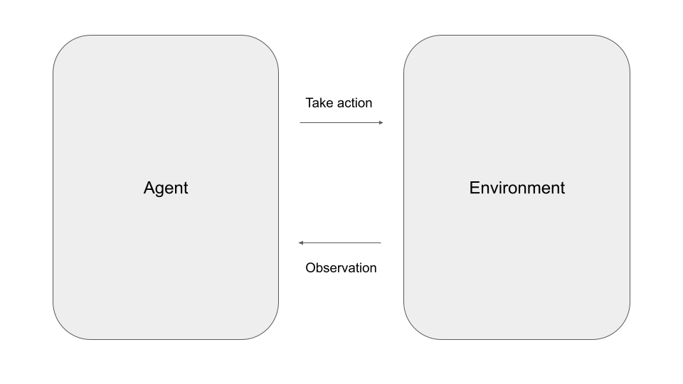
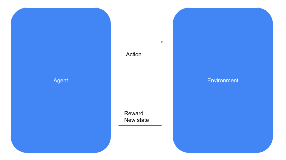
Let us formalize this situation a bit. Reinforcement learning is about an agent like our vacuum cleaning robot that operates in an environment – our apartment – and, at each point in time, has to select one out of a set of possible actions, like moving forward, backward, left or right. When selecting an action, the robot receives a feedback from the environment called a reward, which is simply a scalar value that signals the agent whether the decision it has taken is considered beneficial or not. In our example, for instance, we could give the robot a small positive reward for every square meter it has cleaned, a larger positive reward for reaching the charging station and a small negative reward, i.e. a penalty, when it bumps into a wall.

In every time step, the agent can select one the available actions. The environment will then provide the reward and, in addition, update the state of the system (which, in our case, could be the location of the agent in the apartment and the charging state of the battery). The agent then receives both, the reward and the new state, as an information and proceeds with the next time step.

Let us now look at two ways to formalize this setting – mathematics and code. In mathematical terms, a problem in reinforcement learning is given by the following items. First, there is a set $\mathcal{S}$ of states, which we typically assume to be finite, and a set $\mathcal{A}$ of possible actions, which we assume to be finite as well. In addition, there is a set $\mathcal{R} \subset \mathbb{R}$ of rewards.

The reward that the agent receives for a specific action and the next state depend on the current state and the action. We could now proceed and define this is a mapping

$\mathcal{S} \times \mathcal{A} \rightarrow \mathcal{R} \times \mathcal{S}$

However, in many cases, this assignment has a probabilistic character, i.e. the reward and the next state are not fully deterministic. Therefore, the framework of a Markov decision process (MDP) that we use here describes rewards and next state via a probability distribution conditioned on the current state and the action, i.e. as

$p(S_{t+1} = s', R_{t+1} = r | S_t = s, A_t = a)$

where S_t+1 is the state at time t + 1, S_t is the state at time t, A_t is the action taken at time t and R_t+1 is the reward that the agent receives at time t (this convention for the index of the reward might appear a bit unusual, but is in fact quite common in the field). Collectively, these conditional probabilities are called transition probabilities.

Note that we are making two crucial assumptions here. The first one is that the reward and next state depend only on the action and the current state, not on any previous state and not on the history of events so far (Markov property). This is rather a restriction when modelling a real world problem, not a restriction on the set of problems to which we can apply the framework, as we could simply redefine our state space to be the full history up to the current timestep. Second, we assume that the agent has access to the full state on which rewards and next states depend. There are also more general frameworks in which the agent only receives an observation that reflects a partial view on the actual state (this is the reason why some software packages use the term observation instead of state).

Let us now look at this from a different angle and see how this is modeled as an API. For that purpose, we will look at the API of the popular Gymnasium framework. Here, the central object is an environment that comes with two main methods – step and reset. The method reset resets the environment to an initial state and returns that state. The method step is more interesting. It accepts an action and returns a reward and the new state (called an observation in the Gym framework), exactly as indicated in the diagram above.

Thus an agent that uses the framework would essentially sit in a loop. In every step, it would pick an action that it wants to perform. It would then call the step method of the environment which would trigger the transition into a new state, depending on the action passed as argument. From the returned data, the agent would learn about the reward it has received as well as about the next state.

When would the loop end? This does of course depend on the problem at hand, but many problems are episodic, meaning that at some point in time, a terminal state is reached which is never left again and in which no further rewards are granted. The series of time steps until such a terminal state is reached is called an episode. We will see later than in applications to language modelling, an episode could be a turn in a dialogue or a sentence until an end-of-sentence token is sampled. However, there are also continuing tasks which continue potentially forever. An example could be a robot that learns to walk – there is no obvious terminal state in this task, and we would even encourage the robot to continue walking as long as possible.

Policies and value functions

We have now described a mathematical framework for states and actions. What we have not yet discussed, however, is how the agent actually takes decisions. Let us make the assumption that the agents decisions only depend on the state (and not, for instance, on the time step). The rule which assigns states to actions is called the policy of the agent. Again, we could model this in a deterministic way, i.e. as a function

$\mathcal{S} \rightarrow \mathcal{A}$

but it turns out to be useful to also allow for stochastic policies. A policy is then again a probability distribution which describes the probability that the agent will take a certain action, conditioned on the current state. Thus, a policy is a conditional probability

$\pi(a | s) = \pi(A_t = a | S_t = s)$

Note that given a policy, we can calculate the probability to move into a certain state s’ starting from a state s as

$P(S_{t+1} = s' | S_t = s) = \sum_{a,r} \pi(a | s) p(r, s' | a, s)$

giving us a classical Markov chain.

What makes a policy a good policy? Usually, the objective of the agent is to maximize the total reward. More precisely, for every time step t, the reward R_t+1 at this time step is a random variable of which we can take the expectation value. To measure how beneficial being in a certain state s is, we could now try to use the sum

$\sum_t \mathbb{E}_\pi \left( R_{t+1} | S_0 = s\right)$

of all these conditional expectation values as a measure for the total reward. Note that the conditioning simply means that in order to calculate the expectation values, we only consider trajectories that start at given state s.

However, it is not obvious that this sum converges (and it is of course easy to come up with examples where it does not). Therefore, one usually builds a discounting factor $0 < \gamma < 1$ into this equation and defines the value of a state s to be the conditional expectation value

$v_\pi(s) = \sum_t \gamma^t \mathbb{E}_\pi \left( R_{t+1} | S_0 = s \right)$

Note that the discounting factor plays two roles in this definition. First, it makes sure that under mild conditions, for instance a bound on the rewards, the sum is finite. Second, the value of a reward received early in the trajectory is higher than the value of the same reward at a later time step, so the discounting encourages the agent to collect rewards as early as possible. Whether this is reasonable for the problem at hand is a matter of modelling, and in real implementations, we often see discounting factors close to one.

The mapping that assigns to each state s the value v(s) defined above is called the value function. Note that the expectations are taken with respect to the state transition probabilities given by the policy $\pi$ , and in fact the value function depends on the policy. In general, the objective of the agent will be to find a policy which maximizes the value function for all states or for a distinguished state.

In addition to this value function that assigns a value to a state, there are also two additional functions that we will have to use. First, instead of assigning a value to a state, we could as well assign a value to a state and a given action. This action-value function is usually denoted by q and defined as

$q_\pi(s,a) = \sum_t \mathbb{E}_\pi \left( \gamma^t R_{t+1} | S_0 = s, A_0 = a \right)$

In other words, this is the expected discounted return if we start in state s and choose a as the first action before we start following the policy. Finally, the advantage function

$A_\pi(s, a) = q_\pi(s,a) - v_\pi(s)$

essentially measure the additional benefit (or penalty) of choosing a as action in state s compared to the average under the policy.

PPO

To explain PPO, let us simplify things a bit and assume that we have picked a dedicated starting state s₀ and are aiming at maximizing the outcome for this state only, i.e. we are trying to find a policy that maximizes the value of this state. Suppose that we start with a randomly chosen policy $\pi$ and are striving to identify a better policy $\pi'$ . As a starting point, we can relate the value of our state under the policy $\pi'$ to that under $\pi$ and find, after some calculations that I will not reproduce here and that you can find in [1], that

$v_{\pi'}(s_0) - v_\pi(s_0) = \mathbb{E}_{s \sim \pi'} \left[ \sum_a \pi'(a | s) A_\pi(s, a) \right]$

Here, the expectation value is taken with respect to $\pi'$ , more precisely it is taken with respect to the so-called discounted state distribution defined by $\pi'$ . We will not go through the proof, but intuitively, this makes sense – note that in order to maximize the right-hand side, we need to amplify the probabilities $\pi'(a | s)$ for which the advantage taken with respect to $\pi$ is positive, i.e. those actions which represent an improvement over the current policy $\pi$ .

Let us now suppose that we model the policy $\pi$ using a neural network (spoiler: later, this will be our language model). We could then try to maximize the right hand side of this equation using gradient descent (or rather gradient ascent), and this relation would tell us that by doing so, we would obtain a better policy $\pi'$ . Unfortunately, there are two problems with this – the sampling and the unknown advantage function.

Let us first take a look at the advantage function. To calculate the loss function (or rather objective, as we want to maximize this, not minimize) we need the values of the advantage function. To do this, PPO uses the so-called actor-critic approach: in addition to the model describing the policy (called the actor model) which we want to optimize, we maintain a second model, called the critic, which is trained to learn the value function. We will later see that in each iteration of the PPO algorithm, we sample a few trajectories using the current policy, and during this phase, we can observe the resulting rewards and use them to derive an estimate for the advantage function. This estimate can then be used as ground truth for the critic model and we can apply gradient descent to train the critic model to approximate the advantage function as closely as possible. In practice, the actor model and the critic model have the same architecture and only differ in the top-level layer, or even share layers and weights.

The second problem is more difficult to solve. When looking at the equation above, we see that the policy $\pi'$ – which we want to tune to maximize our objective – appears in two different places, namely inside the sum over the actions but also in the probability distribution that we use to define the expectation value. To estimate the expectation value, we would have to sample from this distribution, but after the first iteration of gradient ascent, we have changed $\pi'$ and all our samples, being taken with the previous value of the weights, would become stale. Even worse, sampling is a non-differentiable operation, so we cannot simply apply a backward pass to calculate the gradient that we need to apply to the weights.

In [1], an algorithm that has become known as TRPO (Trust region policy optimization) was proposed that deals with this problem by making an approximation. Specifically, instead of using the loss function (note the minus sign to be able to use gradient descent)

$\mathcal{L} =- \mathbb{E}_{s \sim \pi'} \left[ \sum_a \pi'(a | s) A_\pi(s, a) \right]$

it uses the loss function

$\mathcal{L} =- \mathbb{E}_{s \sim \pi} \left[ \sum_a \pi'(a | s) A_\pi(s, a) \right]$

Note the subtle but important difference – we take the expectation value with respect to the distribution $\pi$ , not $\pi'$ as before. This approximation turns out to work well as long as $\pi'$ and $\pi$ are not too different (in [1], this is spelled out using the so-called Kullback-Leibler divergence, we will see soon that PPO uses a slightly different approach to enforce this). Trivially, this is the same as

$\mathcal{L} =- \mathbb{E}_{s \sim \pi} \left[ \sum_a \frac{\pi'(a | s)}{\pi(a | s)} \pi(a | s) A_\pi(s, a) \right]$

which we can write as an expectation value over the actions as well, namely

$\mathcal{L} =- \mathbb{E}_{s, a \sim \pi} \left[ \sum_a \frac{\pi'(a | s)}{\pi(a | s)} A_\pi(s, a) \right]$

This is not yet exactly the loss function that PPO actually uses, but let us pause there for a moment and use this preliminary loss function to discuss the overall structure of the algorithm.

First, we initialize both models – the actor model that will learn our policy and the critic model that will learn the value function. Next, we perform the actual training iterations. In each iteration, we go through two phases as indicated in the diagram above – the sampling phase and the optimization phase.

In the sampling phase, we use our current policy $\pi$ to sample a few trajectories until we have collected data from a pre-defined number of state transitions, typically a few hundred or thousand. We do, however, not process these state transitions directly but first store them in a buffer.

One this is done, we enter the second phase, the optimization phase. In this phase, we randomly sample mini-batches from the previously filled buffer. Each item in one of the batches will give us one term of the form

$\frac{\pi'(a | s)}{\pi(a | s)} A_\pi(s, a)$

i.e. one term in the loss function (behind the scenes, we use the critic model and a method known as GAE (see [2]) to calculate the advantage term). We add up these terms for a batch, obtain the loss function and apply a gradient descent step. This will give us new, updated weights of the actor model and therefore a new policy $\pi'$ . Note, however, that the samples are still from the old policy $\pi$ . We then repeat this for a given number of batches and epochs.

At this point, one iteration is complete. We now repeat the procedure for the next iteration, using $\pi'$ as starting policy $\pi$ from which we sample. In each iteration, we obtain a slightly improved policy , and we repeat this until we have reached convergence or a predefined number of iterations.

This already looks like a meaningful approach, but we have ignored one important point. Our loss function is an approximation, which gets worse within each iteration as $\pi'$ starts to deviate significantly from $\pi$ . To solve this, the PPO algorithm proposed in [3], uses the ratio

$r_t = \frac{\pi'(a_t | s_t)}{\pi(a_t | s_t)}$

as a measure for the distance between $\pi'$ and $\pi$ . To control this distance and thus the error that we make by using the approximation for the loss function, PPO clips this ratio, i.e. restricts it to an interval of the form $\left[ 1 - \epsilon, 1 + \epsilon \right]$ where $\epsilon$ is a hyperparameter that is often chosen to be 0.2.. This additional clipping yields the full loss function that PPO uses – in reality, the loss function is even a bit more complicated as the clipping logic depends on the sign of the advantage function and reads as follows.

$- \mathbb{E}_{s, a \sim \pi} \left[ \min( r_t A_{\pi}(s,a) , \mathrm{clip}(r_t, 1 + \epsilon, 1 - \epsilon) A_{\pi}(s,a) ) \right]$

PPO and language models

Having discussed PPO in a more general setting, let us now translate the terminology used in the previous few sections to the world of language models. First, we need to define what states and actions we will use to describe the training of a language model as a problem in reinforcement learning.

Intuitively, our state should correspond to the state of the conversation that a human has with the model. Therefore, a state is given by a prompt (which we would in practice sample from a set of prompts serving as test data) along with a partial completion, i.e. a sequence of token following the prompt. The actions are simply the token in the vocabulary, and the state transition is deterministic and modelled by simply appending the token. Here is an example.

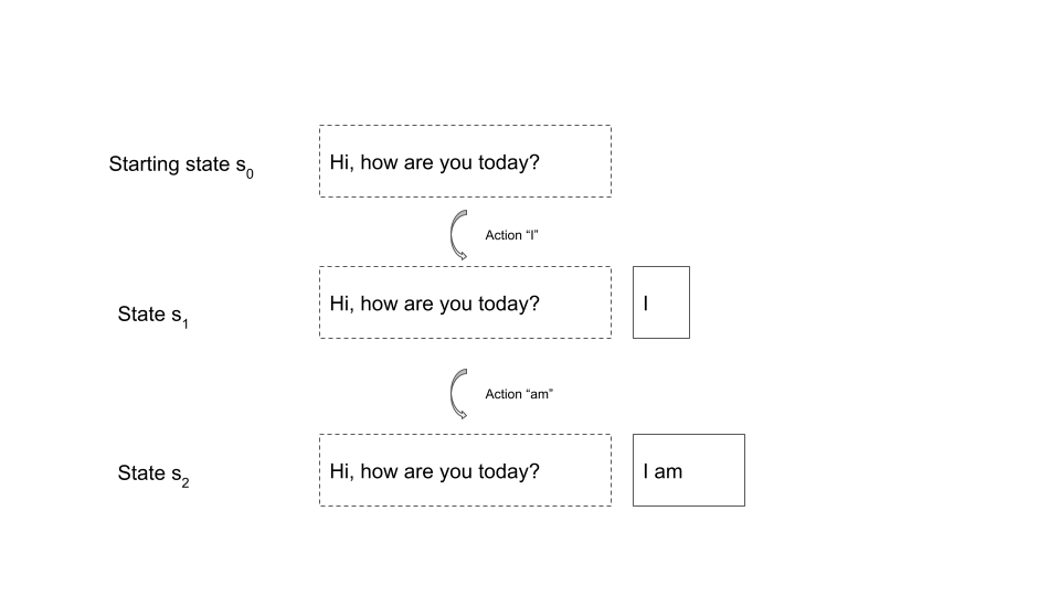
In this case, the initial state is the prompt “Hi, how are you today?”. When we sample a trajectory starting at this state, our first action could be the token “I”. We now append this token to the existing prompt and end up in the state given by the sequence of token “Hi, how are you today? I”. Next, we might sample the token “am” which takes us to the state “Hi, how are you today? I am” and so forth. A state is considered a terminal state if the last token is a dedicated end-of-sentence token used to indicate that the reply of the model is complete. Thus, an episode starts with a prompt and ends with a full reply from the model – in other words, an episode is a turn in the conversation with the model.

With this, it should also be clear what our policy is. A policy determines the probability for an action given a state, i.e. the probability of the next token given a sequence of token consisting of the initial prompt and the already sampled token – and this is of course what a language model does. So our policy is simply the language model we want to train.

To implement PPO, we also need a critic model. We could, for instance, again use a transformer that might or might not share some weights with the policy model, equipped with a single output head that models the value function.

Finally, we need a reward. Recall that the reward function is a (stochastic) function of states and actions. Thus, given an initial prompt x and a partial completion y, of which the last token is the selected action, we want to assign a reward r(x, y). This reward has two parts. The first part is only non-zero if y is complete, i.e. at the end of an episode, and – for reasons that will become clear in a minute – we will denote this part by

$RM(x, y)$

The second part is designed to address the issue that during reinforcement learning, the model might learn a policy that decreases the overall quality of the language model as it deviates too much from the initial model. To avoid this, this second term is a penalty based on the Kullback-Leibler divergence between the current policy and a reference policy $\pi^{ref}$ (if you have never heard the term Kullback-Leibler divergence before, think of it as a distance between two probability distributions). This penalty term is

$- \beta \left[ \ln \frac{\pi'(y | x)}{\pi^{ref}(y | x)} \right]$

where $\beta$ is a hyperparameter which might be dynamically adapted during training.

Let us now talk about the actual reward RM(x, y). In an ideal world, this could be a reward determined by a human labeler that reflects whether the output is aligned with certain pre-defined criteria like accuracy, consistency or the absence of inappropriate language. Unfortunately, this labeling step would be an obvious bottleneck during training and would restrict us to a small number of test data items.

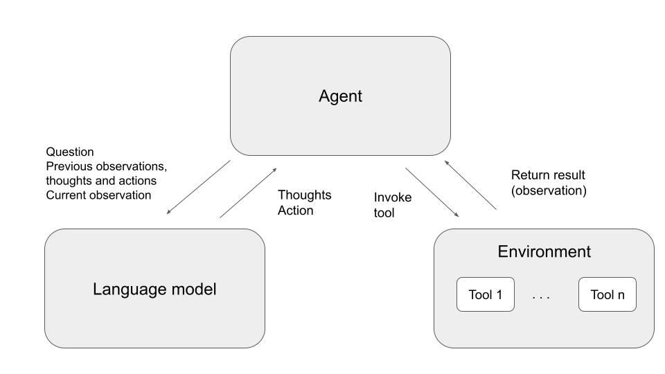
To solve this, OpenAI (building on previous work of other groups) trained a separate model, the so-called reward model, to predict the reward that a human labeler would assign to the reply. This reward model was first trained using labeled test data, i.e. episodes rated by a workforce of human labelers. Then, the output of this model (called RM(x,y) above) was used as part of the reward function for PPO. Thus, there are actually four models involved in the training process, as indicated in the diagram below.

First, there is the model that we train, also known as the actor model or the policy. This is the policy from which we sample, and we also use the probabilities that it outputs as inputs to the loss function. Next, there is, as always when using the PPO algorithm, the critic model which is only used during training and is trained to estimate the value of a state. The reward model acts as a substitute for a human labeler and assigns rewards to complete trajectories, i.e. episodes.

The reference model is a copy of the policy model which is frozen at the beginning of the training. This model is sometimes called the SFT model, where SFT stands for supervised fine tuning, as in the full training cycle used by OpenAI described nicely in this blog post, it is the result of a pretraining on a large data set plus fine tuning on a collection of prompts and gold standard replies created by a human workforce. Its outputs are used to calculate the Kullback-Leibler divergence between the current version of the policy and the reference model. All these ingredients are then put together in the loss function. From the loss function, gradients are derived and the critic as well as the actor are updated.

This completes our discussion of how PPO can be used to align language models with human feedback, an approach that has become known as reinforcement learning from human feedback (RLHF). Even though this is a long post, there are many details that we have not yet covered, but armed with this post and the references below, you should now be able to dig deeper if you want. If you are new to reinforcement learning, you might want to consult a few chapters from [6] which is considered a standard reference, even though I find the mathematics a bit sloppy at times, and then head over to [1] and [3] to learn more about PPO. If you have a background in reinforcement learning, you might find [3] as well as [4] and [5] a good read.

This post is also the last one in my series on large language models. I hope I could shed some light on the mathematics and practical methods behind this exciting field – if yes, you are of course invite to check out my blog once in a while where I will most likely continue to write about this and other topics from machine learning.

References

[1] J. Schulman et. al, Trust Region Policy Optimization, available as arXiv:1502.05477
[2] J. Schulman et al., High-Dimensional Continuous Control Using Generalized Advantage Estimation, available as arXiv:1506.02438
[3] J. Schulman et al., Proximal Policy Optimization Algorithms, available as arXiv:1707:06347
[4] D. Ziegler et al., Fine-Tuning Language Models from Human Preferences}, available as arXiv:1909.08593
[5] N. Stiennon et al., Learning to summarize from human feedback, available as arXiv:2009.01325
[6] R. S. Sutton, A.G. Barto, Reinforcement learning – an introduction, available online here

Mastering large language models – Part XVI: instruction fine-tuning and FLAN-T5

In most of our previous posts, we have discussed and used transformer networks that have been trained on a large set of data using teacher forcing. These models are good at completing a sentence with the most likely next token, but are not optimized for following instructions. Today, we will look at a specific family of networks that have been trained to tailor their response according to instructions – FLAN-T5 by Google.

If you ask a language model that has been trained on a large data set to complete a prompt that represents an instruction or a question, the result you will obtain is the most likely completion of the prompt. This, however, might not be the answer to your question – it could as well be another question or another instruction, as the model is simply trying to complete your prompt. For many applications, this is clearly not what we want.

One way around this is few-shot learning which basically means that you embed your instruction into a prompt that somehow resembles the first few lines of a document so that the answer that you expect is the most natural completion, giving the model a chance to solve your task by doing what it can do best, i.e. finding completions. This, however, is not really a satisfying approach and you might ask whether there is a way to fix the problem at training time, not at inference time. And in fact there is a method to train a model to recognize and follow instructions – instruction fine-tuning.

Most prominent models out there like GPT did undergo instruction fine tuning at some point. Today we will focus on a model series called FLAN-T5 which has been developed by Google and for which the exact details of the training process have been published in several papers (see the references). In addition, versions of the model without instruction fine tuning are available so that we can compare them with the fine-tuned versions.

In [1], instruction fine-tuning has been applied to LaMDA-PT, a decoder-only transformer model that Google had developed and trained earlier. In [2], the same method has been applied to T5, a second model series presented first in [3]. The resulting model series is known as FLAN-T5 and available on the Hugginface hub. So in this post, we will first discuss T5 and how it was trained and than explain the instruction fine tuning that turned T5 into FLAN-T5.

T5 – an encoder-decoder model

Other than most of the models we have played with so far, T5 is a full encoder-decoder model. If you have read my previous post on transformer blocks and encoder-decoder architectures, you might remember the following high-level overview of such an architecture.

For pre-training, Google did apply a method known as masking. This works as follows. Suppose your training data contains the following sentence:

The weather report predicted heavy rain for today

If we encode this using the the encoder used for training T5, we obtain the sequence of token

[37, 1969, 934, 15439, 2437, 3412, 21, 469, 1]

Note that the last token (with ID 1) is the end-of-sentence token that the tokenizer will append automatically to our input. We then select a few token in the sentence randomly and replace each of them with one of 100 special token called extra_id_NN, where NN is a number between 0 and 99. These token have IDs ranging from 32000 to 32099, where 32099 is extra token 0 and 32000 is extra token 99. After applying this procedure known as masking our sentence could look as follows

The weather report predicted heavy <extra_id_0> for today

[37, 1969, 934, 15439, 2437, 32099, 21, 469, 1]

We now train the decoder to output a list of the extra token used, followed by the masked word. So in our case, the target sequence for the decoder would be

<extra_id_0> rain

or, again including the end-of-sentence token

[32099, 3412, 1]

In other words, we ask our model to guess the word that has been replaced by the mask (this will remind you of the word2vec algorithm that I have presented in a previous post). To train the combination of encoder and decoder to reach that objective, we can again apply teacher forcing. For that purpose, we shift the labels to the right by one and append a special token called the decoder start token to the left (which, by the way, is identical to the padding token 0 in this case). So the input to the decoder is

[0, 32099, 3412]

We then can calculate the cross-entropy loss between the decoder output and the labels above and apply gradient descent as usual. I have put together a notebook for this post that walks you through an example and that you can also run on Google Colab as usual.

Pre-training using masking was the first stage in training T5. In a second stage, the model was fine-tuned on a set of downstream tasks. Examples for these tasks include translation, summarization, question answering and reasoning. For each task, the folks at Google defined a special format in which the model received the inputs and in which the output was expected. For translation, for instance, the task started with

“translate English to German: “

followed by the sentence to be translated, and the model was trained to reply with the correct translation. Another example is MNLI, which is a set of pairs of premise and hypothesis, and the model is supposed to answert with one word indicating whether a premise implies the hypothesis, is a contradiction to it or is neutral towards the hypothesis. In this case, the input is a sentence formatted as

“mnli premise: … premise goes here… hypothesis: … hypothesis goes here…

and the model is expected to answer with one of the three words “entailment”, “contradiction” or “neutral”. So all tasks are presented to the model as pure text and the outcome is expected to be pure text. My notebook contains a few examples of how this works.

From T5 to FLAN-T5

After the pre-training using masking and the fine-tuning, T5 is already a rather powerful model, but still is sometimes not able to deduce the correct task to perform. In the notebook for this post, I hit upon a very illustrative example. If we feed the sentence

Please answer the following question: what is the boiling temperature of water?

into the model, it will not reply with the actual boiling point of water. Instead, it will fall back to one of the tasks it has been trained on and will actually translate this to German instead of answering the question.

This is where instruction fine-tuning [2] comes into play. To teach the model to recognize instructions as such and to follow them, the T5 model was trained on a large number of additional tasks, phrased in natural language.

To obtain a larger number of tasks from the given dataset, the authors applied different templates to each task. If, for instance, we are given an MNLI task with a hypothesis H and a premise P, we could present this in several ways to the model, i.e. according to several templates. We could, for instance, turn the data point into natural language using the template

“Premise: P. Hypothesis: H. Does the premise entail the hypothesis?”

Or we could phrase this as

Based on the premise P, can we conclude that the hypothesis H is true?

By combining every data point from the used data set with a certain number of templates, a large dataset for the fine-tuning was obtained, and the model learned to deal with many different instructions referring to the same type of task, which hopefully would enable the model to infer the correct tasks for an unseen template at test time. As Google published the code to generate the data, you can take a look at the templates here.

Also note that the data contains some CoT (chain-of-thought) prompting, i.e. some of the instruction templates for reasoning tasks include phrases like “apply reasoning step-by-step” to prepare the model for later chain-of-thought prompting.

In the example in my notebook, the smallest FLAN-T5 model (i.e. T5 after this additional fine-tuning procedure) did at least recognize that the input is a question, but the reply (“a vapor”) is still not what we want. The large model does in fact reply with the correct answer (212 F).

Instruction fine-tuning has become the de-facto standard for large language models. The InstructGPT model from which ChatGPT and GPT-4 are derived, however, did undergo an additional phase of training – reinforcement learning from human feedback. This is a bit more complex, and as many posts on this exist which unfortunately do only scratch the surface I will dive deeper into this in the next post which will also conclude this series.

References

[1] J. Wei et al., Finetuned Language Models Are Zero-Shot Learners, arXiv:2109.01652
[2] H.W. Chung et al., Scaling Instruction-Finetuned Language Models, arXiv:2210.11416
[3] C. Raffel et al., Exploring the Limits of Transfer Learning with a Unified Text-to-Text Transformer, arXiv:1910.10683

Mastering large language models Part XV: building a chat-bot with DialoGPT and Streamlit

Arguably, a large part of the success of models like GPT is the fact that they have been equipped with a chat frontend and proved able to have a dialogue with a user which is perceived as comparable to a dialogue you would have with another human. Today, we will see how transformer based language models can be employed for that purpose.

In the previous post, we have seen how we can easily download and run pretrained transformer models from the Huggingface hub. If you play with my notebook on this a bit, you will soon find that they do exactly what we expect them to do – find the most likely completion. If, for instance, you use the promt “Hello”, followed by the end-of-sentence token tokenizer.eos_token, they will give you a piece of text starting with “Hello”. This could be, for instance, a question that someone has posted into a Stackexchange forum.

If you want to use a large language model to build a bot that can actually have a conversation, this is usually not what you want. Instead, you want a completion that is a reply to the prompt. There are different ways to achieve this. One obvious approach that has been taken by Microsoft for their DialoGPT model is to already train the model (either from scratch or via fine-tuning) on a dataset of dialogues. In the case of DialoGPT, the dataset has been obtained by scraping from Reddit.

A text-based chat-bot

Before discussing how to use this model to implement a chat-bot, let us quickly fix a few terms. A conversation between a user and a chat-bot is structured in units called turns. A turn is a pair of a user prompt and a response from the bot. DialoGPT has been trained on a dataset of conversations, modelled as a sequence of turns. Each turn is a sequence of token, where the user prompt and the reply of the bot are separated by an end-of-sentence (EOS) token. Thus a typical (very short) dialogue with two turns could be represented as follows

Good morning!<eos>Hi<eos>How do you feel today?<eos>I feel great<eos>

Here the user first enters the prompt “Good morning!” to which the bot replies “Hi”. In the second turn, the user enters “How do you feel today” and the bot replies “I feel great”.

Now the architecture of DialoGPT is identical to that of GPT-2, so we can use what we have learned about this class of models (decoder-only models) to sample from it. However, we want the model to take the entire conversation that took place so far into account when creating a response, so we feed the entire history, represented as a sequence of token as above, into the model when creating a bot response. Assuming that we have a function generate that accepts a prompt and generates a reply until it reaches and end-of-sentence token, the pseudocode for a chat bot would therefore look as follows.

input_ids = []
while True:
    prompt = input("User:")
    input_ids.extend(tokenizer.decode(prompt))
    input_ids.append(tokenizer.eos_token)
    response = generate(input_ids)
    print(f"Bot: {tokenize.decode(response)}"
    input_ids.extend(response)

Building a terminal-based chat-bot on top of DialoGPT is now very easy. The only point that we need to keep in mind is that in practice, we will want to cache past keys and values as discussed in the last post. As we need the values again in the next turn which will again be based on the entire history, our generate function should return these values and we will have to pass them back to the function in the next turn. An implementation of generate along those lines can be found here in my repository. To run a simple text-based chatbot, simply do (you probably want to run this in a virtual Python environment):

git clone https://github.com/christianb93/MLLM
cd MLLM
pip3 install -r requirements.txt
cd chatbot
python3 chat_terminal.py

The first time you run this, the DialoGPT model will be downloaded from the hub, so this might take a few minutes. To select a different model, you can use the switch --model (use --show_models to see a list of valid values).

Using Streamlit to build a web-based chat-bot

Let us now try to build the same thing with a web-based interface. To do this, we will use Streamlit, which is a platform designed to easily create data-centered web applications in Python.

The idea behind Streamlit is rather simple. When building a web-based applicaton with Streamlit, you put together an ordinary Python script. This script contains calls into the Streamlit library that you use to define widgets. When you run the Streamlit server, it will load the Python script, execute it and render an HTML page accordingly. To see this in action, create a file called test.py in your working directory containing the following code.

import streamlit as st 


value = st.slider(label = "Entropy coefficient", 
          min_value = 0.0, 
          max_value = 1.0)
print(f"Slider value: {value}")

Then install streamlit and run the applications using

pip3 install streamlit==1.23.1 
streamlit run test.py

Now a browser window should open that displays a slider, allowing you to select a parameter between 0 and 1.

In the terminal session in which you have started the Streamlit server, you should also see a line of output telling you that the value of the slider is zero. What has happened is that Streamlit has started an HTTP server listening on port 8501, processed our script, rendered the slider that we have requested, returned its current value and then entered an internal event loop outside of the script that we have provided.

If now change the position of the slider, you will see a second line printed to the terminal containing the new value of the slider. In fact, if a user interacts with any of the widgets on the screen, Streamlit will simply run the script once more, this time returning the updated value of the slider. So behind the scenes, the server is sitting in an event loop, and whenever an event occurs, it will not – like frontend frameworks a la React will do it – use callbacks to allow the application to update specific widgets, but instead run the entire script again. I recommend to have a short look at the section “Data flow” in the Streamlit documentation which explains this in a bit more detail.

This is straightforward and good enough for many use cases, but for a chat bot, this creates a few challenges. First, we will have to create our model at some point in the script. For larger models, loading the model from disk into memory will take some time. If we do this again every time a user interacts with the frontend, our app will be extremely sluggish.

To avoid this, Streamlit supports caching of function values by annotating a function with the decorator st.cache_resource. Streamlit will then check the arguments of the function against the cached values. If the arguments match a previous call, it will directly return a reference to the cached response without actually invoking the function. Note that here a reference is returned, meaning in our case that all sessions share the same model.

The next challenge that we have is that our application requires state, for instance the chat history or the cached past keys and values, which we have to preserve for the entire session. To maintain session-state, Streamlit offers a dictionary-like object st.session_state. When we run the script for the first time, we can initialize the chat history and other state components by simply adding a respective key to the session state.

st.session_state['input_ids'] = []

For subsequent script iterations, i.e. re-renderings of the screen, that are part of the same session, the Streamlit framework will then make sure that we can access the previously stored value. Internally, Streamlit is also using the session state to store the state of widgets, like the position of a slider or the context of a text input field. When creating such a widget, we can provide the extra parameter key which allows us to specify the key under which the widget state is stored in the session state.

A third feature of Streamlit that turns out to be useful is to use conventional callback functions associated with a widget. This makes it much easier to trigger specific actions when a specific widget changes state, for instance if the user submits a prompt, instead of re-running all actions in the script every time the screen needs to be rendered. We can, for instance, define a widget that will hold the next prompt and, if the user hits “Return” to submit the prompt, invoke the model within the callback. Inside the callback function, we can also update the history stored in the session state.

def process_prompt():
    #
    # Get widget state to access current prompt
    #
    prompt = st.session_state.prompt
    #
    # Update input_ids in session state
    #
    st.session_state.input_ids.extend(tokenizer.encode(prompt))
    st.session_state.input_ids.append(tokenizer.eos_token_id)
    #
    # Invoke model
    #
    generated, past_key_values, _ = utils.generate(model = model, 
                                            tokenizer = tokenizer, 
                                            input_ids = st.session_state.input_ids, 
                                            past_key_values = st.session_state.past_key_values, 
                                            temperature = st.session_state.temperature, debug = False)
    response = tokenizer.decode(generated).replace('<|endoftext|>', '')
    #
    # Prepare next turn
    #
    st.session_state.input_ids.extend(generated)

Armed with this understanding of Streamlit, it is not difficult to put together a simple web-based chatbot using DialoGPT. Here is a screenshot of the bot in action.

You can find the code behind this here. To run this, open a terminal and type (switching to a virtual Python environment if required):

git clone https://github.com/christianb93/MLLM
cd MLLM
pip3 install -r requirements.txt
cd chatbot
streamlit run chat.py

A word of caution: by default, this will expose port 8501 on which Streamlit is listening on the local network (not only on localhost) – it is probably possible to change this somewhere in the Streamlit configuration, but I have not tried this.

Also remember that the first execution will include the model download that happens in the background (if you have not used that model before) and might therefore take some time. Enjoy your chats!

Mastering large language models – Part XIV: Huggingface transformers

In the previous post, we have completed our journey to being able to code and train a transformer-based language model from scratch. However, we have also seen that in order to obtain professional results, we need an enormous amount of resources, i.e. training data and compute power. Luckily, there are some pre-trained transformer models that we can use, be it directly for inference or as a basis for further fine-tuning. Today, we will take a look at the probably most prominent platform that exists for that purpose – the Huggingface platform.

Huggingface is a company that offers a variety of services around machine learning. In our context, we will mainly be interested in the wo of their products – the transformers library and the Huggingface hub, which is a platform to which scientists and enthusiasts can upload weights and trained models to make them available for everyone using the Huggingface transformer library.

As a starting point, let us first make sure that we have the library installed. For this post (and the entire series) I have used version 4.27.4, which you can install as usual.

pip3 install transformers==4.27.4

The recommended starting point for working with the library is a pipeline, which is essentially a container that includes everything which we typically need, most notably a tokenizer and a model. As the intention of this post, however, is to make contact with the models which we have implemented so far, we will dig a bit deeper and start directly with a model instead.

In the transformers library, pretrained models are usually downloaded from the hub and identified by name, which – by convention – is the name of the provider followed by a slash and the name of the model. Here is a short code snippet that you can execute in a notebook or in an interactive Python session which will download the weights for the 1.3 billion parameter version of the GPT-Neo model. GPT-Neo is a series of models developed and trained by EleutherAI and made available as open source, including the weights.

import transformers
import torch
model_name="EleutherAI/gpt-neo-1.3B"
model = transformers.AutoModelForCausalLM.from_pretrained(model_name)
print(model)
print(isinstance(model, torch.nn.Module))

Executing this for the first time will trigger the download of the model to ~/.cache/huggingface/hub. The entire download is roughly 5 GB MB, so this might take a second. If you want to avoid the large download, you can also use the much smaller 125m version – just change the last part of the model name accordingly. From the output, we can see that this model is a torch.nn.Module, so we can use it as any other PyTorch model.

We can also see that the model actually consists of two components, namely an instance of the class GPTNeoModel defined here and a linear layer – the so-called head – that is sitting on top of the actual transformer and, as usual, transforms between the model inner dimension which is 2048 and the one-hot encoded vocabulary. This decomposition of the full model into a core model and a task-specific head is common to most Huggingface models, as it allows us to use the same set of weights for different tasks.

Even though the model does not use the transformer blocks that are part of PyTorch, it is a decoder-only transformer model as we would expect it – there are two learned embeddings for positions and words and 24 transformer blocks consisting of self-attention and linear layers. There is a minor difference, though – every second layer in the GPT-Neo model uses local self-attention, which basically means that to calculate the attention at a given position, only keys and values within a sliding window are used, not all keys and values in the context – see the comment here.

Apart from this, our model is very close to the models that we have implemented and trained previously. We know how to sample from such a model. But before we can do this, we need to turn our attention to the second part of a pipeline, namely the tokenizer.

Obviously, a pretrained transformer model will only produce reasonable results if we use the same vocabulary and the same tokenizer for inference that we have used for training. Therefore, the Huggingface hub contains a matching tokenizer for every pretrained model. This tokenizer can be downloaded and initialized similar to what we have done for the model.

tokenizer = transformers.AutoTokenizer.from_pretrained(model_name)

Our tokenizer will contain everything that we need to convert forth and back between text and sequences of token. Specifically, the main components of a tokenizer are as follows.

First, there is method encode which accepts a text and returns a sequence of token IDs, and a method decode which conversely translates a sequence of token IDs into a text.

To convert between the string representation of a token and the ID, there are the methods convert_ids_to_tokens and convert_tokens_to_ids. In addition, the tokenizer obviously contains a copy of the vocabulary and some special token like a token that marks the end of a sentence (EOS token), the beginning of a sentence (BOS token), unknow token and so forth – this should in general match the token defined in the model config model.config

In our case, the tokenizer is an instance of the GPT2 tokenizer which in turn is derived from the PretrainedTokenizer class.

Having a tokenizer at our disposal, we can now sample from the model in exactly the same way as from our own models. There are two little details that we need to keep in mind. First, in the Huggingface world, the batch dimension is the first dimension. Second, the forward method of our model returns a dictionary in which the logits are stored under a key with the same name. Also, the context size is part of the model config and called max_position_embeddings. Thus our sampling method looks as follows, assuming that we have a method do_p_sampling that draws from a distribution p.

def predict(model, prompt, length, tokenizer, temperature = 0.7,  p_val = 0.95):
    model.eval()
    with torch.no_grad():
        sample = []
        device = next(model.parameters()).device
        #
        # Turn prompt into sequence of token IDs
        # 
        encoded_prompt  = tokenizer.encode(prompt)        
        encoded_sample = encoded_prompt
        encoded_prompt = torch.tensor(encoded_prompt, dtype = torch.long).unsqueeze(dim = 0)
        with torch.no_grad():
            out = model(encoded_prompt.to(device)).logits # shape B x L x V
            while (len(encoded_sample) < length):
                #
                # Sample next character from last output. Note that we need to remove the
                # batch dimension to obtain shape (L, V) and take the last element only
                #
                p = torch.nn.functional.softmax(out[0, -1, :] / temperature, dim = -1)
                #
                # Sample new index and append to encoded sample
                #
                encoded_sample.append(do_p_sampling(p, p_val))
                #
                # Feed new sequence
                #
                input = torch.tensor(encoded_sample[-model.config.max_position_embeddings:], dtype=torch.long)
                input = torch.unsqueeze(input, dim = 0)
                out = model(input.to(device)).logits
                print(tokenizer.decode(encoded_sample))

        return tokenizer.decode(encoded_sample)

This works, but it is awfully slow, even on a GPU. There is a reason for that, which is similar to what we have observed when sampling from an LSTM.

Suppose that our prompt has length L, and that we have already sampled the first token after the prompt, so that our full sample now has length L + 1. We now want to sample the next token. For that purpose, we only need the logits at position L + 1, so it might be tempting to feed only token L + 1 into our model. Let us quickly recall why this does not work.

To derive the output at position L + 1, each attention block will run the attention value at position L + 1 (which is a tensor of shape B x V) through the feed-forward network. If q denotes the query at position L + 1, this attention value is given by

$\frac{1}{\sqrt{d}} \sum_{i=0}^{L} (q \cdot k_i) v_i$

So we see that we need all keys and values to calculate the attention – which is not surprising, as this is the way how the model takes the context into account – but the query is only needed for position L + 1 (which is index 0, as we use zero-based indexing). Put differently, the only reason why we need to feed the previously generated token again and again into the model is that we need to key and value pairs from the past.

This hints at an opportunity to speed up inference – we could try to cache these values. To realize this, the Huggingface model returns the keys and values of all layers as an item past_key_values in the output and allows us to provide this as an additional argument to the next call. Thus instead of passing the full tensor of input IDs of length L + 1, we can as well pass only the last value, i.e. the ID of the currently last token, plus in addition the key value pairs from the previous call. Here is the updated sampling function.

def predict(model, prompt, length, tokenizer, temperature = 0.7,  p_val = 0.95):
    model.eval()
    with torch.no_grad():
        sample = []
        device = next(model.parameters()).device
        #
        # Turn prompt into sequence of token IDs
        # 
        encoded_prompt  = tokenizer.encode(prompt)        
        encoded_sample = encoded_prompt
        input_ids = torch.tensor(encoded_prompt, dtype = torch.long).unsqueeze(dim = 0)
        with torch.no_grad():
            #
            # First forward pass- use full prompt
            #
            out = model(input_ids = input_ids.to(device))
            logits = out.logits[:, -1, :] # shape B x V
            past_key_values = out.past_key_values
            while (len(encoded_sample) < length):
                #
                # Sample next character from last output
                #
                p = torch.nn.functional.softmax(logits[0, :] / temperature, dim = -1)
                #
                # Sample new index and append to encoded sample
                #
                idx = do_p_sampling(p, p_val)
                encoded_sample.append(idx)
                #
                # Feed new token and old keys and values
                #
                input_ids = torch.tensor(idx).unsqueeze(dim = 0)
                out = model(input_ids = input_ids.to(device), past_key_values = past_key_values)
                logits = out.logits
                past_key_values = out.past_key_values
                print(tokenizer.decode(encoded_sample))

        return tokenizer.decode(encoded_sample)

This should be significantly faster and provide a decent performance even on a CPU – when running this, you will also realize that the first pass that feeds the entire prompt takes some time, but all subsequent passes are much faster.

That closes our post for today. We have bridged the gap between the models that we have implemented and trained so far and the – much more advanced – models on the Huggingface hub and have convinced ourselves that even though these models are of course much larger and more powerful, their architecture is the same as for our models, and we can use them in the same way. I encourage you to play with a few other models which can be sampled from in exactly the same way, like the Pythia models from EleutherAI or the gpt2-medium and gpt2-large versions of the GPT model that can all be found on the Huggingface hub – you can use the code snippets from this post or my notebook as a starting point.

In the next post, we will use the popular Streamlit platform to implement a simple ChatBot backed by a Huggingface model.

Mastering large language models – Part XIII: putting it all together

Today, we will apply what we have learned in the previous posts on BPE, attention and transformers h- we will implement and train a simple decoder-only transformer model from scratch.

First, let us discuss our model. The overall structure of the model is in fact quite similar to the model we have used when training an LSTM on “War and Peace” – we will have an embedding layer turning words into vectors, the actual network and an output layer of the dimension of the vocabulary from which we will sample our next word. However, there are a few notable differences.

The most obvious and most important one is that we use a transformer instead of an LSTM. More specifically, we will use a decoder-only model, i.e. there is no input from an encoder. Instead, the model applies self-attention on the input in each layer. Recall that technically, the transformer blocks in this model will be instances of torch.nn.TransformerEncoderLayer even though we will use them as decoder building blocks. We will also have to use masking to avoid that our model can peek ahead in the self-attention layers.

The second difference is that instead of character-level encoding, we will apply a BPE tokenizer trained with a fixed number of merges. We will use sinusoidal positional embeddings as in the original transformer paper. With these modifications, our model looks as follows.

Using the sinusoidal embeddings discussed in one of our previous posts, we can now easily code our model in Python.

class Model(torch.nn.Module):
    
    def __init__(self, vocab_size, model_dim = MODEL_DIM, context_size = CONTEXT_SIZE, ff_dim = FF_DIM, heads = HEADS, layers = LAYERS, dropout = DROPOUT):
        super().__init__()
        self._word_embedding = torch.nn.Embedding(vocab_size, model_dim)
        self._pe_embedding = PosEmbeddingLayer(context_size, model_dim)
        layer = torch.nn.TransformerEncoderLayer(d_model = model_dim, nhead = heads, dim_feedforward = ff_dim, dropout = dropout)
        self._transformer = torch.nn.TransformerEncoder(layer, num_layers = layers)
        self._linear = torch.nn.Linear(in_features = model_dim, out_features = vocab_size)
        self._model_dim = model_dim
        self._context_size = context_size
        self._vocab_size = vocab_size
        cached_mask = torch.tril(torch.ones(context_size, context_size)*(-1)*float('inf'), diagonal = -1).t()
        self.register_buffer("_cached_mask", cached_mask)
    
    #
    # Create a causal self-attention mask
    #
    def get_self_attention_mask(self):
        return self._cached_mask
        
    #
    # Shape of input: (L, B)
    # 
    def forward(self, x):
        assert len(x.shape) == 2, "Expecting two-dimensional input"
        (L, B) = x.shape
        x = self._word_embedding(x) # shape (L, B, model_dim)
        x = self._pe_embedding(x) 
        #
        # Mask input. As we have registered this is a buffer, it
        # should already be on the same device as the model
        #
        mask = self.get_self_attention_mask()[:L, :L]
        x = self._transformer(x, mask = mask)
        return self._linear(x)

Note the causal self-attention mask that we use. In order to avoid having to recalculate this mask for every input, we create the mask once and add it as a buffer to the model, which will ensure that the mask will also be transferred if we move our model to the GPU.

We also follow the convention to use the second dimension as batch dimension. So our initial input will have shape (L, B), where each column of length L is a tensor whose elements are the indices of a token in the vocabulary, which we then pass through the embedding layers to obtain a tensor of shape (L, B, D). We then pass this through all transformer layers and finally through the output layer which will project this back into the vocabulary, i.e. we now have a tensor of shape (L, B, V). As usual, we do not include the final softmax, so that we have to apply the softmax before we sample.

Let us now discuss our dataset and the preprocessing. As for our word2vec example, we will use the WikiText dataset. This dataset comes in two flavors: WikiText2 with a bit more than 2 million token and WikiText103 with a bit more than 100 million token. During preprocessing, we need to pre-tokenize the dataset, build a BPE vocabulary and a rule set from it, encode the data and finally split it into a training dataset and a validation dataset. Training then proceeds as usual using teacher forcing. As in the GPT-3 paper, we use a cosine learning rate schedule to decrease the learning rate over time from its original value by 90%.

If you want to train the model from scratch but do not have access to a CUDA-enable machine, you can play with the notebook that I have created for this post on Google CoLab. For this notebook, I use the smaller WikiText2 dataset and train for only three epochs. The runtime does of course depend on the GPU (and the CPU) that Google will assign to your runtime. When I tried this, running the BPE merge and encoding the entire dataset took roughly 5 minutes in total, and the training took less than 30 minutes.

Here is a short sample created using the model trained on Google CoLab (which you can also find in the notebook itself).

Federer also received the first title of the Australian Open in the finals, including the Madonna Open, the Duke of Florence, and his first tournament. Federer won the final, losing to the finals, having scored a record nine times to five consecutive weeks before losing 19, in the Bir ‘Shoot , an injury

Of course this does not really make sense, but is still a bit impressive for less than 30 minutes of training. Most parts of this sentence are grammatically meaningful, and some snippets do even sound reasonable.

To get better results, we can try to train the model on a larger dataset, for instance the full WikiText103 data set instead of the small WikiText2 dataset. This goes beyond what we can reasonably do with a free GPU on Google CoLab. If, however, you have access to a decent GPU, you can do the training yourself. To create the training dataset, run the following commands (after activating a matching Python environment as described in the README)

#
# Clone repository if not yet done
#
git clone https://github.com/christianb93/MLLM
cd MLLM/wiki
#
# Remove existing data and run preprocessing
#
rm -f vocab.dat rules.data data.json
python3 preprocess.py

This takes a few minutes as we will have to build a BPE vocabulary and encode the entire dataset (do not trust the initial ETCs during encoding – as we implement a cache, the speed will go up with every word already decoded, and the entire process should take around 15 – 20 min, depending of course on your environment). The results of the preprocessing are five files – the vocabulary vocab.dat, the merge rules rules.dat, the fulll encoded dataset data.json as well as files train.json and val.json for training and validation (if the vocabulary, rules and data file exist, they will be reused, so make sure to remove existing copies if you do not want this).

Once the preprocessing is complete, we can start the training. I trained the model for two epochs on an A10 machine on Lambdalabs, using the command

python3 train.py --epochs=2 --compile --autocast

On this machine, one batch took 0.05 seconds, resulting in a runtime of 7.5 hours for two epochs. I have added the resulting model checkpoint model.pt to the repository (make sure to delete this file if you want to train from scratch, as otherwise training will restart from this file).

We can now sample from the model (either from the pretrained model or from a model from a custom training run) by simply running

python3 predict.py

By default, this will apply nucleus sampling with p=0.95 and a temperature of 0.7. Here is an output generated using the pretrained model that is part of the repository.

His wedding did not hear the explanation of the title, as his term ” Alan Keegan ” was in a press release. The first episode was broadcast on July 13, 2007. The episode was written by Matt Groening, and was written by Stella Packard. The episode was broadcast on BBC One in the United States on July 11, 2009, and was watched by 2. 93 million viewers, and it was watched by 7. 50 million viewers in the United States. It was the first time that the episode was viewed by 4. 21 million viewers and was viewed by 4. 3 million households. The episode received a 3. 1 rating / 9 share among viewers between the ages of 18 and 49. The episode was watched by approximately 7. 8 million viewers. It received generally positive reviews from television critics. It received generally positive reviews from television critics, according to Nielsen Media Research…

The first sentence does not make too much sense, but the second and the next few sentences do at least make partial sense. We also see, however, that the model tends to repeat itself, which is probably due to the comparatively low temperature. Here is another sample generated with temperature 0.9.

The series was a single nine – part series against Ivor on its official website. Two seasons earlier, the original series was released on May 2, 2014, was released as a partnership with Clifton Notes in the United States. These were a number of reprint edition hardcover footage. Many reviews were positive and negative and positive. Loves made Yerne the first film in the series by Dirty, featuring Beyoncé ‘s voice acting. The lead character Ron Fisk of Hope called the film ” a rogue look inside “. Lyrically, the crew got off in a course at the end of the scene. Sacred Kimball, who played by the actors of the film, left England at the end of the episode, was shot in a short story of a movie about that film. The film was influenced by David Duchovny

Clearly, this is still not GPT – on the other hand, our model is tiny (it has only roughly 5 million parameters, compared to the 175 billion parameters used for GPT-3) and so is our data (a bit more than 100 million token, whereas GPT-3 was trained on more than 300 billion token). Theoretically, we could now proceed to train larger models on more data, but the cost associated with the required infrastructure will soon become prohibitive.

Fortunately, a few models and weights are available to the public. Probably the easiest way to download and run these models is the Huggingface Transformers library. In our next post, we will start to work with this library to download popular models like GPT-2 and play with them.

Mastering large language models – Part XII: byte-pair encoding

On our way to actually coding and training a transformer-based model, there is one last challenge that we have to master – encoding our input by splitting it in a meaningful way into subwords. Today, we will learn how to do this using an algorithm known as byte-pair encoding (BPE).

Let us first quickly recall what the problem is that subword encoding tries to solve. To a large extent, the recent success of large language models is due to the tremendous amount of data used to train them. GPT-3, for instance, has been trained on roughly 500 mio tokens (which, as we will see soon, are not exactly words) [3]. But even much smaller datasets tend to contain a large number of unique words. The WikiText103 dataset [4] for instance contains a bit more than 100 mio. words, which represent a vocabulary of 267.735 unique words. With standard word-level encoding, this would become a dimension in the input and output layers of our neural network. It is not hard to imagine that with 500 mio. token as input, this number would even be much larger and we clearly have a problem.

The traditional way to control the growth of the vocabulary is to introduce a minimum frequency. In other words, we could only include token in the vocabulary that occur more than a given number of times – the minimum frequency – in the training data and tune this number to realize a cap on the vocabulary size. This, however, has the disadvantage that during training and later inference, we will face unknown words. Of course we can reserve a special token for these unknown words, but still a translator would have to know how to handle them.

Character-level encoding solves the problem of unknown words, but introduces a new problem – the model first has to learn words before it can start to learn relations between words. In addition, if our model is capable of learning relations within a certain range L, it does of course make a difference whether the unit in which we measure this range is a character or a word.

This is the point where subword tokenization comes into play. Here, the general idea is to build up a vocabulary that consists of subword units, not full words – but also more than just individual characters. Of course, to make this efficient, we want to include those subwords in our vocabulary that occur often, and we want to include all individual characters. If we need to encode a word that consists of known subwords, we can use those, and in the worst case, we can still go down to the character level during encoding so that we will not face unknown words.

Byte-pair encoding that has first been applied to machine learning in [1] is one way to do this. Here, we build our vocabulary in two phases. In the first phase, we go through our corpus and include all characters that we find in our vocabulary. We then encode our data using this preliminary vocabulary.

In the second phase, we iterate through a process known as merge. During each merge, we go through our data and identify the pair of token in the vocabulary that occurs most frequently. We then include a new token in our vocabulary that is simply the concatenation of these two existing token and update our existing encoding. Thus every merge adds one more token to the vocabulary. We continue this process until the vocabulary has reached the desired size.

Note that in a real implementation, the process of counting token pairs to determine their frequency is usually done in two steps. First, we count how often an individual word occurs in the text and save this for later reference. Next, given a pair of token, we go through all words that contain this pair and then add up the frequencies of these words to determine the frequency of the token pair.

Let us look at an example to see how this works in practice. Suppose that the text we want to encode is

low, lower, newest, widest

In the first phase, we would build an initial vocabulary that consists of all characters that occur in this text. However, we want to make sure that we respect word boundaries, so we need to be able to distinguish between characters that appear within a word and those that appear at the end of the word. We do this by adding a special token </w> to a token that is located at the end of a word. In our case, this applies for instance to the character w that therefore gives rise to two entries in our vocabulary – w and w</w>. With this modification, our initial vocabulary is

'o', 'r</w>', 's', 'w</w>', 'n', 'i', 'e', 'l', 'd', 'w', 't</w>'

We now go through all possible combinations of two token and see how often the appear in the text. Here is what we would find in our example.

Token pair	Frequency
l + o	2
o + w</w>	1
o + w	1
w + e	2
e + r</w>	1
n + e	1
e + w	1
e + s	2
s + t</w>	2
w + i	1
i + d	1
d + e	1

We now pick the pair of token (usually called a byte-pair, even though this is strictly speaking of course not correct when we use Unicode points) that occurs most frequently. In our case, several byte pairs occur twice, and we pick one of them, say w and e. We now add an additional token “we” to our vocabulary and re-encode our text. With this vocabulary, our text which previously was represented by the sequence of token

l, o, w</w>, l, o, w, e, r</w>, n, e, w, e, s, t</w>, w, i, d, e, s, t</w>

would now be encoded as

l, o, w</w>, l, o, we, r</w>, n, e, we, s, t</w>, w, i, d, e, s, t</w>

Note the new token, marked with bold face, that appears at the two positions where we previously had the combination of the token w and e. This concludes our first merge.

We can now continue and conduct the next merge. Each merge will add one token to our vocabulary, so that controlling the number of merges allows us to create a vocabulary of the desired size. Note that each merge results in two outputs – an updated vocabulary and a rule. In our case, the first merge resulted in the rule w, e ==> we.

To encode a piece of text that was not part of our training data when running the merges, we now simply replay these rules, i.e. we start with our text, break it down into characters, corresponding to the token in the initial vocabulary, and apply the rules that we have derived during the merges in the order in which the merges took place. Thus to encode text, we need access to the vocabulary and to the rules.

Let us now turn to implementing this in Python. The original paper [1] does already contain a few code snippets that make an implementation based on them rather easy. As usual, this blog post comes with a notebook that, essentially based on the code in [1], guides you through a simple implementation using the example discussed above. Here are a few code snippets to illustrate the process.

The first step is to build a dictionary that contains the frequencies of individual words, which we will later use to easily calculate the frequency of a byte pair. Note that the keys in this dictionary are the words in the input text, but already broken down into a sequence of token, separated by spaces, so that we need to update them as we merge and add new token.

def get_word_frequencies(pre_tokenized_text):
    counter = collections.Counter(pre_tokenized_text)
    word_frequencies = {" ".join(word) + "</w>" : frequency for word, frequency in counter.items() if len(word) > 0}
    return word_frequencies

As the keys in the dictionary are already pretokenized, we can now build our initial vocabulary based on these keys.

def build_vocabulary(word_frequencies):
    vocab = set()
    for word in word_frequencies.keys():
        for c in word.split():
            vocab.add(c)
    return vocab

Next, we need to be able to identify the pair of bytes that occurs most frequently. Again, Python collections can be utilized to do this – we simply go through all words, split them into symbols, iterate through all pairs and increase the count for this pair that we store in a dictionary.

def get_stats(word_frequencies):
  pairs = collections.defaultdict(int)
  for word, freq in word_frequencies.items():
    symbols = word.split()
    for i in range(len(symbols)-1):
      pairs[symbols[i],symbols[i+1]] += freq
  return pairs

Finally, we need a function that executes an actual merge. During each merge, we use regular expressions (more on the exact expression that we use here can be found in my notebook) to replace each occurence of the pair by the new token.

def do_merge(best_pair, word_frequencies, vocab):
    new_frequencies = dict()
    new_token = "".join(best_pair)
    pattern = r"(?<!\S)" + re.escape(" ".join(best_pair)) + r"(?!\S)"
    vocab.add(new_token)
    for word, freq in word_frequencies.items():
        new_word = re.sub(pattern, new_token, word)
        new_frequencies[new_word] = word_frequencies[word]
    return new_frequencies, vocab

We can now combine the functions above to run a merge. Essentially, during a merge, we need to collect the statistics to identify the most frequent pair, call our merge function to update the dictionary containing the word frequencies and append the rule that we have found to a list of rules that we will save later.

stats = get_stats(word_frequencies)
best_pair = max(stats, key=lambda x: (stats[x], x)) 
print(f"Best pair: {best_pair}")
word_frequencies, vocab = do_merge(best_pair, word_frequencies, vocab)
rules.append(best_pair)

This code, howevers, is awfully slow, as it basically repeats the process of counting once with every merge. The authors of the original paper also provide a reference implementation [2] that applies some tricks like caching and the use of indices to speed up the process significantly. In my repository for this series, I have assembled an implementation that follows this reference implementation to a large extent, but simplifies a few steps (in particular the incremental updates of the frequency counts) and is therefore hopefully a bit easier to read. The code consists of the main file BPE.py and a test script test bpe.py.

The test script can also be used to compare the output of our implementation with the reference implementation [3]. Let us quickly do this using a short snippet from “War and peace” that I have added to my repository.

#
# Clone the reference implementation
#
git clone https://github.com/rsennrich/subword-nmt.git
cd subword-nmt
#
# Get files from my repository
#
wget https://raw.githubusercontent.com/christianb93/MLLM/main/bpe/BPE.py
wget https://raw.githubusercontent.com/christianb93/MLLM/main/bpe/test_bpe.py
wget https://raw.githubusercontent.com/christianb93/MLLM/main/bpe/test.in
wget https://raw.githubusercontent.com/christianb93/MLLM/main/bpe/test.rules
#
# Run unit tests
# 
python3 test_bpe.py
#
# Run reference implementation
#
cat test.in | python3 subword_nmt/learn_bpe.py -s=50 > rules.ref
#
# Run our implementation
#
python3 test_bpe.py --infile=test.in --outfile=rules.dat
#
# Diff outputs
#
diff rules.dat rules.ref
diff rules.ref test.rules

The only difference that the diff should show you is a header line (containing the version number) that the reference implementation adds which we do not include in our output, all the remaining parts of the output files which contain the actual rules should be identical. The second diff verifies the reference file that is part of the repository and is used for the unit tests.

Over time, several other subword tokenization methods have been developed. Two popular methods are Googles wordpiece model ([6], [7]) and the unigram tokenizer [8]. While wordpiece is very similar to BPE and mainly differs in the way how the next byte pair for merging is selected, the unigram tokenizer starts with a very large vocabulary, containing all characters and the most commonly found substrings, and then iteratively removes items from the vocabulary based on a statistic model.

With BPE, we now have a tokenization method at our disposal which will allow us to decouple vocabulary size from the size of the training data, so that we can train a model even on large datasets without having to increase the model size. In the next post, we will put everything together and train a transformer-based model on the WikiText dataset.

References:

[1] R. Sennrich et al., Neural Machine Translation of Rare Words with Subword Units
[2] https://github.com/rsennrich/subword-nmt
[3] T. Brown et al., Language Models are Few-Shot Learners
[4] https://blog.salesforceairesearch.com/the-wikitext-long-term-dependency-language-modeling-dataset/
[5] K. Bostrom, G. Durrett, Byte Pair Encoding is Suboptimal for Language Model Pretraining
[6] Y. Wu et al., Google’s Neural Machine Translation System: Bridging the Gap between Human and Machine Translation
[7] M. Schuster, K. Nakajima, Japanese and Korean voice search
[8] T. Kudo, Subword Regularization: Improving Neural Network Translation Models with Multiple Subword Candidates

Autonomous agents and LLMs: AutoGPT, Langchain and all that

Over the last couple of months, a usage pattern for large language models that leverages the model for decision making has become popular in the LLM community. Today, we will take a closer look at how this approach is implemented in two frameworks – Langchain and AutoGPT.

One of the most common traditional use cases in the field of artificial intelligence is to implement an agent that operates autonomously in an environment to achieve a goal. Suppose, for instance, that you want to implement an autonomous agent for banking that is integrated into an online banking platform. This agent would communicate with an environment, consisting of the end user, but maybe also backend systems of the bank that would allow it to gather information, for instance on account balances, and to trigger transactions. The goal of the agent would be to complete a customer request.

In a more abstract setting, an agent operates in discrete time steps. At each time step, it receives an observation – which, in the example above, could be a user input or the result of a call into the backend system – and can decide to take one out of a list of available actions, like making a new request to a backend system or completing the conversation with the end user – a formalism that you will have seen before if you have ever studied reinforcement learning. So the task of the agent is to select the next action, depending on the current and potentially on previous observations.

Obviously, there are many different possibilities to implement an agent – and, maybe not surprisingly, one approach that has been applied successfully in the recent past is to use a large language model as the brain of our agent. The idea behind this approach is to feed the observations, encoded as plain text, into the model at each step and to ask the model for the next action to take.

In practice, this can be done using few-shot learning, i.e. we generate a prompt for our model that consists of a few examples that inform the model about the format that we expect and the possible actions, and then add the last actual observation as a final prompt. To allow our model to take all previous observations into account, we would always include the full trajectory of observations and actions into the model.

In this paper, an approach termed ReACT (Reasoning and acting) has been proposed to orchestrate a large language model for decision making. In this framework, the environment is modelled as a set of tools that the agent can utilize. In the original paper, there are actually three tools corresponding to three different actions that the agent can take. First, it can retrieve a summary from Wikipedia. Second, it can lookup details on the Wikipedia page to which it has navigated with the first action, and finally it can complete the task and return the final result.

In each step, the agent now asks the model what action it should take next. It then runs one of the available tools to execute the action and adds the result as new observation to the next prompt that it sends to the model. To improve the quality of the results, a prompt engineering technique known as chain-of-thought prompting (CoT) is used, which basically means that the prompt contains an instruction for the model to spell out its thoughts, i.e. the rationale for the proposed action. Thus each prompt consists of the original question to be answered and the full history of thoughts, actions and observations.

Here is an example generated by the Langchain implementation of an agent following the ReACT pattern. For a better understanding, I have marked the output of the model in italic.

Question: Out of the following three countries, only two are direct neighbors of France: Germany, Spain, Poland. Please name the country in the list which is not a neighbor of France
Thought: I need to search France, find its neighbors, then find the country in the list which is not a neighbor of France
Observation: France, officially the French republic, is a country located primarily … (long summary of the Wikipedia artice on France)
Thought: France has neighbors such as Germany, Spain, Belgium, Luxemburg, Switzerland, Italy, Monaco, Andorra and the United Kingdom. So the country in the list which is not a neighbor of France is Poland.
Action: Finish[Poland]

To encourage the model to follow this pattern and to use only the allowed actions, the Langchain implementation uses few-shot learning, i.e. the prompt contains a few examples that follows this scheme (you can find these examples here, these are actually the examples cited in the original paper). So the full prompt consists of the few-shot examples, followed by the question at hand and the full sequence of observations, thoughts and actions generated so far.

Let us take a short look at the implementation in Langchain. These notes have been compiled using version 0.202. As the toolset seems to be evolving quickly, some of this might be outdated when you read this post, but I am confident that the basic ideas will remain.

First, Langchain distinguishes between an agent which is the entity talking to the language model, and the agent executor which talks to the agent and runs the tools.

The AgentExecutor class implements the main loop indicated in the diagram above. In each iteration, the method _take_next_step first invokes the agent, which will in turn assemble a prompt as explained above and generate a response from the language model. The output is then parsed and returned as an AgentAction which also contains the thought that the model has emitted. Then, the tool which corresponds to the action is executed and its output is returned along with the selected action.

Back in the main loop, we first test whether the action is an instance of the special type AgentFinish which indicates that the task is completed and we should exit the main loop. If not, we append the new tuple consisting of thought, action and observation to the history and run the next iteration of the loop. The code is actually quite readable, and I highly recommend to clone the repository and spend a few minutes reading through it.

Let us now compare this to what AutoGPT is doing. In its essence, AutoGPT uses the same pattern, but there are a few notable differences (again, AutoGPT seems to be under heavy development, at the time of writing, version 0.4.0 is the stable version and this is the version that I have used).

Similar to the ReACT agent in Langchain, AutoGPT implements an agent that interacts with an LLM and a set of tools – called commands in AutoGPT – inside a main loop. In each iteration, the agent communicates with the AI by invoking the function chat_with_ai. This function assembles a prompt and generates a reply, using the OpenAI API in the background to talk to the selected model. Then, the next action is determined based on the output of the model and executed (in the default settings, the user is asked to confirm this action before running it). Finally the results are added to the history and the next iteration starts.

The first difference compared to the ReACT agent in Langchain is how the prompt is structured. The prompt used by AutoGPT consists of three sections. First, there is a system prompt which defines a persona, i.e. it instructs the model to embody an agent aiming to achieve a certain set of goals (which are actually generated via a separate invocation of the model initially and saved in a file for later runs) and contains further instructions on the model. In particular, the system prompt instructs the model to produce output in JSON format as indicated below.

{
    "thoughts": {
        "text": "thought",
        "reasoning": "reasoning",
        "plan": "- short bulleted- list that conveys- long-term plan",
        "criticism": "constructive self-criticism",
        "speak": "thoughts summary to say to user"
    },
    "command": {
        "name": "command name",
        "args": {
            "arg name": "value"
        }
    }
}

This is not only much more structured than the simple scheme used in the ReACT agent, but also asks the model to express its thoughts in a specific way. The model is asked to provide additional reasoning, to maintain a long-term plan as opposed to simply deciding on the next action to take and to perform self-criticism. Note that in contrast to ReACT, this is pure zero-shot learning, i.e. no examples are provided.

After the system prompt, the AutoGPT prompt contains the conversation history and finally there is a trigger prompt which is simply hardcoded to be “Determine exactly one command to use, and respond using the JSON schema specified previously:“.

Apart from the much more complex prompt using personas and a more sophisticated chain-of-thought prompting, a second difference is the implementation of an additional memory. The idea behind this is that for longer conversations, we will soon reach a point where the full history does not fit into the context any more (or it does, but we do not want to do this as the cost charged for the OpenAI API depends on the number of token). To solve this, AutoGPT adds a memory implemented by some external data store (at the time of writing, the memory system of AutoGPT is undergoing a major rewrite, so what follows is based on an analysis of earlier versions and a few assumptions).

The memory is used in two different places. First, when an iteration has been completed, an embedding vector is calculated for the results of the step, i.e. the reply of the model and the result of the executed command. The result is then stored in an external datastore, which can be as simple as a file on the local file system, but can also be a cache like Redis, and indexed using the embedding.

When an iteration is started, the agent uses an embedding calculated from the last few messages in the conversation to look up the most relevant data in memory, i.e. the results of previous iterations that have the most similar embeddings. These results are then added to the prompt, which gives the model the ability to remember previous outcomes and reuse them in a way not limited by the length of the prompt. This approach of enriching the prompt with relevant information obtained via a semantic search is sometimes called retrieval augmentation – note however that in this case, the information in the data store has been generated by model and agent, while retrieval augmentation usually leverages pre-collected data.

Finally, the AutoGPT agent can choose from a much larger variety of tools (i.e. commands in the AutoGPT terminology) than the simple ReACT agent which only had access to Wikipedia. On the master branch, there are currently commands to run arbitrary Python code, to read and write files, to clone GitHub repository, to invoke other AIs like DALL-E to generate images, to search Google or to even browse the web using Selenium. AutoGPT can also use Elevenlabs API to convert model output to speech.

AutoGPT and ReACT are not the only shows in town – there is for instance BabyAGI that lets several agents work on a list of tasks which are constantly processed, re-prioritized and amended. Similarly, HuggingGPT [7] initially creates a task list that is then processed, instead of deciding on the next action step by step (AutoGPT is an interesting mix between these approaches, as it has a concrete action for the next step, but maintains a global plan as part of its thoughts). It is more than likely that we will see a rapid development of similar approaches over the next couple of months. However, when you spend some time with these tools, you might have realized that this approach comes with a few challenges (see also the HuggingGPT paper [7] for a discussion).

First, there is the matter of cost. Currently, OpenAI charges 6 cent per 1K token for its largest GPT-4 model (and this is only the input token). If you consume the full 32K context size, this will already be 2$ per turn, so if you let AutoGPT run fully autonomously, it could easily spend an amount that hurts in a comparatively short time.

Second, if the model starts to hallucinate or to repeat itself, we can easily follow a trajectory of actions that takes us nowhere or end up in a loop. This has already been observed in the original ReACT paper, and I had a similar experience with AutoGPT – asking for a list of places in France to visit, the agent started to gather more and more detailed information and completely missed the point where I would have been happy to get an answer compiled out of the information that it already had.

Last but not least the use of autonomous agents that execute Python code, access files on your local system, browse the web using your browser and your IP address or even send mails and trigger transactions on your behalf can soon turn into a nightmare in terms of security, especially given that the output of commands ends up in the next prompt (yes, there is something like a prompt injection, see [8] and [9]). Clearly, a set of precautions is needed to make sure that the model does not perform harmful or dangerous actions ([6] provides an example where AutoGPT was starting to install updated SSL certificates to solve a task that a straight-forward web scraping could have solved as well).

Still, despite of all this, autonomous agents built on top of large language models are clearly a very promising approach and I expect to see more powerful, but also more stable and reliable solutions being pushed into the community very soon. Unitl then, you might want to read some of the references that I have assembled that discuss advanced prompting techniques and autonomous agents in more details.

References:

[1] S. Yao et al., ReAct: Synergizing Reasoning and Acting in Language Models, arXiv:2210.03629
[2] Prompt Engineering guide at https://www.promptingguide.ai/
[3] N. Shinn et al., Reflexion: Language Agents with Verbal Reinforcement Learning, arXiv:2303.11366
[4] L. Wang et al., Plan-and-Solve Prompting: Improving Zero-Shot Chain-of-Thought Reasoning by Large Language Models, arXiv:2305.04091
[5] Ask Marvin – integrate AI into your codebase
[6] https://www.linkedin.com/pulse/auto-gpt-promise-versus-reality-rick-molony – an interesting experience with AutoGPT
[7] Y. Shen, HuggingGPT: Solving AI Tasks with ChatGPT and its Friends in Hugging Face, arXiv:2303.17580 – also known as JARVIS
[8] C. Anderson, https://www.linkedin.com/pulse/newly-discovered-prompt-injection-tactic-threatens-large-anderson/
[9] OWASP Top 10 for LLM Security

Mastering large language models – Part XI: encoding positions

In our last post, we have seen that the attention mechanism is invariant to position, i.e. that reordering of the words in a sentence yields the same output, which implies that position information is lost. Clearly position information does matter in NLP, and therefore transformer based models apply positional embeddings in addition to the pure word embeddings.

Before explaining positional embeddings, let us first recall word embeddings in general. Suppose we are working with sentences consisting of L token taken out of a fixed vocabular. Then creating vectors out of these token amounts to map each token

$token_1, token_2, token_3, \dots, token_L$

to a vector v_i. This encoding, however, is usually position independent, meaning that if the same token appears at two different positions in the sentence, the resulting vector will be the same for both instances of the token. Technically, the embedding can be described by a matrix of dimension (D, V), where D is the model dimension and V is the size of the vocabulary, and each column in this matrix represents the embedding for one token.

In the original transformer paper [1], these word embeddings are augmented by an additional positional embedding. Similar to word embeddings, this again attaches a vector of dimension D to every token in the input. However, this embedding now solely depends on the position of the token, and not on the actual token itself, so that different token at the same position yield the same embedding. This additional embedding is then added to the word embedding to obtain one vector per token which is then fed into the actual model.

But what is the vector that we want to add to the word embedding at position i? Obviously, there are many choices (reference [3] is a good survey of existing approaches). The approach taken in the original transformer is to use fixed values which are not learned and not modified during training and are given by the equations

$\textrm{PE}(p, i) = \begin{cases} \sin(C^{i / D} p) & i \, \textrm{even} \\ \cos(C^{(i-1) / D} p) & i \, \textrm{odd} \end{cases}$

where C is a fixed constant (actually 1 / 10000), p is the position of the token in the sentence and i is the vector index, so that PE_p or PE(p, : ) in Python notation is the vector added to the word embedding of a token at position p. Here we assume that the model dimension D is an even number.

The motivation provided for this specific choice in [1] is that for a fixed offset k, the positional encoding vectors PE_p+k and PE_p are related by a linear transformation, so that, as the authors phrase it in section 3.5 of [1], “it would allow the model to easily learn to attend by
relative positions“. Let us quickly verify this. For any i, component 2i of the vector PE_p+k is given by

$\begin{aligned}PE_{p+k, 2i} &= \sin(C^{2i / D} (p+k)) \\ &= \sin(C^{2i/D}p) \cos(C^{2i/D}k) + \cos(C^{2i/D}p) \sin(C^{2i/D}k) \\ &= \cos(C^{2i/D}k) PE_{p,2i} + \sin(C^{2i/D}k) PE_{p,2i+1} \end{aligned}$

and similarly, the component 2i+1 is given by

$\begin{aligned} PE_{p+k,2i+1} &= \cos(C^{2i / D} (p+k)) \\ &= \cos(C^{2i / D}p)\cos(C^{2i / D}k) - \sin(C^{2i / D}p)\sin(C^{2i / D}k) \\ &= \cos(C^{2i / D}k)PE_{p,2i+1} - \sin(C^{2i / D}k)PE_{p,2i} \end{aligned}$

proving our claim. Note that these two relations can nicely be organized into one equation as

$\begin{pmatrix} PE_{p+k, 2i} \\ PE_{p+k, 2i+1} \end{pmatrix} = \begin{pmatrix} \cos(C^{2i / D}k) & \sin(C^{2i / D}k) \\ - \sin(C^{2i / D}k) & \cos(C^{2i / D}k) \end{pmatrix} \begin{pmatrix} PE_{p, 2i} \\ PE_{p, 2i+1} \end{pmatrix}$

showing that the two vectors are related by a rotation (we will get back to this point later when we talk about relative embeddings).

Let us quickly see how we could code this in Python. As we need one embedding vector of dimension D for each position, the embeddings form a matrix of shape (L, D), where each row represents one position. After applying the word embeddings to an input sequence of length L, this will as well result in a matrix of shape (L, D), and we can simply add these two matrices together. Of course, we would not calculate the sine and cosine values above again for every input, but store them in a global variable, an attribute or (better) in a PyTorch buffer. Here is a piece of code to calculate the embeddings, taken from the corresponding section in d2l.ai (note that this only works if D is even, which, however, is usually the case – in fact, dimensions are often multiples of 8, 16 or 32 to better support the inner workings of modern GPUs).

#
# Values for p and 2*i / D
#
_p = torch.arange(L , dtype=torch.float32).unsqueeze(dim = 1)
_i = torch.arange(0, D , step = 2) / D
#
# x = C**(2i/D)*p
#
x = torch.pow(C, _i) * _p
#
# Apply sine and cosine and organize into a matrix pe
#
pe = torch.zeros(L, D)
pe[:, 0::2] = torch.sin(x)
pe[:, 1::2] = torch.cos(x)

For more on this and a few visualisations, you might want to take a look at the notebook for this post.

Note that at this point, we need to make an assumption on the maximum length of the input sequence that we will be using, called the context size. The context size is also an important parameter for training and inference, as the attention matrices have shape (L, L), so that a large context size increases memory usage and computational complexity.

As already mentioned, this way to construct embeddings is not the only one. A second method that has gained some popularity and is for instance applied in GPT-models ([4]) is to use learned embeddings. With this approach, the positional embeddings are treated similarly to the word embeddings, i.e. they are simply parameters that are initialized with some random values and then updated during backward passes as any other parameter of the network.

Both the sinusoidal embeddings used in the original transformer paper as well as the learned embeddings used by GPT are absolute embeddings, i.e. the value of an embedding depends on the absolute position of a token in a sentence. In [2], a different approach is taken which is known as relative embeddings and relies on a modification of the self-attention mechanism to incorporate positional information rather than on absolute positional embeddings added to the word embeddings before processing them in the attention layer.

More specifically, when calculating attention scores and before applying the softmax, the usual dot product between query at position i and key at position j is modified by adding a bias vector w to the key that depends on the relative position, i.e. the difference j – i.

$q \left( \cdot k^t + w_{j-i}\right)$

These bias vectors are then learned, similar to the word embeddings. This modification is applied not only in the first layer, but in all layers. In addition, to avoid having to learn 2*L embeddings for each layer and each attention head, the authors clip the relativ position, i.e. instead of using the index j – i which can range from -L to L, the use the modified index

$\max(-k, \min(k, j-i))$

so that the relative position is clipped to values between -k and k, where k is a hyperparameter. For an efficient implementation, see [5].

Many variations of this approach are possible. An interesting example is the T5 model described in [6] which we will look at in more detail in a later post. In this model, the position dependent vector added to the key before taking the dot product with the query is replaced by a scalar added after taking the dot product, so that the dot product is replaced by

$q \cdot k^t + a_{j-i}$

where a_j-i is now a scalar. These scalars are again learned parameters, shared between different layers but unique for each head. Instead of a clipping, buckets are formed, each corresponding to a range of different values of j – i. so that the number of parameters that need to be learned is simply the number of buckets times the number of heads. It is instructive to take a look at the T5 implementation of the Huggingface Transformer library to see how this works in practice – the notebook for this post contains a simplified and commented version of this code.

Before moving on, let us quickly discuss another type of relative positional embeddings known as rotary embeddings, originally proposed in [7]. In contrast to the approaches that we have seen so far, this method does not modify the self-attention score by adding a vector or scalar, but by rotating queries and keys before forming the dot product. Specifically, the authors consider a set of orthogonal matrices

$R_{\Theta, i}$

depending on a fixed parameter Θ and the position i and replace the usual attention dot product between query and key by

$q_i R_{\Theta, i} (k_j R_{\Theta, j})^t = q_i R_{\Theta, i} R_{\Theta, j}^t k_j^t$

At the first glance, this does not seem to be a relative embedding, as it seems to depend on both positions – the position i of the query and the position j of the key. However, the authors choose a set of matrices that mathematically speaking form something resembling a one-parameter subgroup, i.e. having the property that

$R_{\Theta, i} R_{\Theta, j}^t = R_{\Theta, i - j}$

so that the attention score is actually

$q_i R_{\Theta, i - j} k_j^t$

which does in fact only depend on the difference i – j, i.e. on the relative position of query and key. Rotary embeddings have also been applied in the GPT-NeoX model by EleutherAI.

We now have a broad selection of different embedding methods to our disposal and could go ahead and apply them to train a transformer-based decoder-only model. However, there is still some challenge that we have not touched upon – the word encodings. So far, our word encodings were straightforward – we did either chose to turn each individual character into a token or used word-based encodings where our vocabulary consists of all words found in the training data. Unfortunately, both approaches have certain drawbacks. Character-based encodings imply that the model also has to learn how to assemble words from characters and makes learning long-range relations more difficult. Word-based encodings suffer from the problem that the number of unique words in the training data can become huge, which will blow up our model size.

For that reason, many models use a third approach known as subword tokenization, where token are built from parts of words instead of individual characters or entire words. In the next post, we will therefore study the tokenization mechanism used by the original transformer – byte-pair encoding (BPE).

References:

[1] A. Vaswani et al., Attention is all you need
[2] P. Shaw et al., Self-Attention with Relative Position Representations
[3] P. Dufter, M. Schmitt, H. Schütze; Position Information in Transformers: An Overview. Computational Linguistics 2022; 48 (3): 733–763
[4] A. Radford et al., Improving Language Understanding by Generative Pre-Training
[5] C. Huang et al, Music Transformer: generating music with long-term structure
[6] C. Raffel et al., Exploring the Limits of Transfer Learning with a Unified
Text-to-Text Transformer
[7] J. Su et al., RoFormer: Enhanced Transformer with Rotary Position Embedding

Mastering large language models – Part X: Transformer blocks

Today, we will start to look in greater detail at the transformer architecture. At the end of the day, a transformer is built out of individual layers, the so-called transformer blocks, stacked on top of each other, and our objective for today is to understand how these blocks are implemented.

Learning about transformer architectures can be confusing. If you read the original paper Attention is all you need by Vaswani et al. (and I highly recommend to actually take a look at the paper), you will, already on page 3, stumble upon a rather complicated diagram which is actually a bit intimidating if all of this is new to you. This paper talks about encoders and decoders, which is a language that we understand thanks to a previous post. On the other hand, you will hear statement that popular models like GPT-2 are in fact decoder-only models, without having a clear definition at hand what this actually means. To make things worse, decoder-only models are built out of PyTorch modules which, confusingly enough, are called torch.nn.TransformerEncoder. So before getting into too many details, let us first try to clean up that mess a bit.

The most general transformer models like the one described in the original paper or popular models like T5 are in fact encoder-decoder models. The general architecture is not so much different from the encoder-decoder models that we have already seen in the context of RNNs. There is a first network, the encoder, which translates a source sentence into a sequence of embeddings. Then, there is a second network that uses the output of the encoder as a context – typically called the memory in transformer-based architectures – to generate the source sequence. A crucial difference, though, is that the decoder reads the input of the encoder via an attention layer which gives the decoder network access to all time steps of the encoder at the same time. So very high-level, the picture is as follows.

Let us now dig a bit deeper. In fact, both, the encoder and the decoder, are built out of layers called transformer blocks. For the encoder, every transformer block has one input and one output. For the decoder, every transformer block has two inputs and one output. One input reads, via an attention mechanism, data from the encoder (more precisely, keys and values are taken from the encoder, while queries are taken from the decoder). The second input is taken from the previous transformer block of the encoder. So on the next level of detail, the diagram looks like this.

This explain the first (and most important) architectural difference between an encoder transformer block (torch.nn.TransformerEncoderLayer in PyTorch) and a decoder transformer block (torch.nn.TransformerDecoderLayer) – a decoder block has two inputs, an encoder block only one.

The second difference is the attention mask. Attention is actually applied at all inputs of a transformer block. For an encoder, masking is typically not done, so that the encoder can look at all token in the input. For the decoder, masking is also usually not done for the attention layer connecting the encoder and the decoder, so that the decoder has access to all time steps of the encoder output. For the second attention layer of a decoder, however, connected to the decoder input or the input of the previous layer, a causal self-attention mask is usually applied, i.e. the decoder is not allowed to peak ahead, as discussed in the last post. This difference, however, is not hardcoded into the PyTorch classes, as the attention mask in PyTorch is a parameter.

Finally, there are decoder-only transformers, and this is the class of transformer on which we will focus in the next few posts. These are transformers that are built from encoder blocks, each of which receives only one input, so there is no encoder. However, the attention mask used for the input is the one used for the decoder, so that we can apply teacher forcing to train such a model. Thus a decoder-only transformer receives a sequence of length L as input, encoded as a matrix of shape (L, D) where D is the embedding dimension, and produces an output of the same shape. If we add an embedding layer and an output layer, we can apply such a model for language generation very much in the same manner as an RNN, and this is the use case we will study first.

So let us talk about transformer blocks (more specifically, transformer blocks with only one input, i.e. encoder blocks in the PyTorch terminology) in more detail. Instead of jumping directly to the paper, let us take a different approach and look at the source code of the corresponding PyTorch module. The key lines in the forward method are

 x = self.norm1(x + self._sa_block(x, src_mask, src_key_padding_mask))
 x = self.norm2(x + self._ff_block(x))

Let us see what this does. First, we feed the input through a self-attention block. Note, however, that it is on us to specify a causal attention mask, as the model will not do this automatically.

Next, we apply a residual connection, i.e. we take the output of the self attention and add the original input to it. This helps to avoid vanishing gradients, as it allows a part of the gradient during backpropagation to flow directly back to the previous layer. Finally, we apply a layer normalization to the output, i.e. to the sum.

We then repeat the same pattern. This time, however, we run the result of the previous step through a feed-forward network before we again add the input to establish a residual connection and finally apply a normalization. Thus our full flow looks as follows.

So we repeat the pattern

$\textrm{LayerNorm}(x + \textrm{Sublayer}(x))$

twice, where first the sublayer is a self-attention layer and then the sublayer is a feed-forward network. This is, in fact, exactly the expression that we find in section 3.1 of the original paper.

Before we proceed, let us talk about dimensions. When working with transformers, it is common to present the input in the format (L, B, D), where L is the sequence length, B is the batch size and D is the dimension of the model. Each sublayer produces an output of the same shape, and so does the layer norm, so that the entire transformer block again produces an output of that shape.

In addition, a more careful look a the code shows that at the output of each sublayer, there is a dropout layer to avoid overfitting. As usual, the dropout is deactivated during inference and evaluation, but active during training.

So far, so good, but we are still missing an important point in our overall approach. To spot this, let us go ahead and quickly try out a transformer block in PyTorch, then permute the token in the input, i.e. change the orders of the input vectors, and run the new input through the transformer block again. Here is a short piece of code doing this (you can also have a look at the notebook that I prepared for this post.

# Model dimension
D = 8
# Length of encoder input
L = 4
#
# Create random input
#
X = torch.randn(L, D)
#
# and feed through an encoder block
#
block = torch.nn.TransformerEncoderLayer(d_model = D, nhead = 4)
block.eval()
Y = block(X).detach()
#
# Now permute the input, recompute
#
Xp = X.flip(dims = [0]).detach()
Yp = block(Xp).detach()
#
# Verify that Yp is simply the permutation of Y
#
print(f"{torch.allclose(Yp, Y.flip(dims = [0]))}")

We find that permuting the input to a transformer simply results in the same permutation applied to the output. This is not surprising after a closer look at the formula for the attention, but is not really matching our intuition of a good encoding of a sentence. After all, the two sentences

The dog chases the cat

and

The cat chases the dog

are permutations of each other, but have completely different meanings, so that from a good encoding, we would expect more than just a permutation as well. The problem becomes even more apparent if we now simulate the first step of processing that encoder output in a decoder, i.e. passing it through the attention layer connecting encoder and decoder. Recall that this attention layer uses keys and values from the encoder output, but the queries from the decoder input. Let us simulate this.

# length of target sequence, i.e. decoder input
T = 3 
queries = torch.randn(T, D)
attn = torch.nn.MultiheadAttention(embed_dim = D, num_heads = 4)
#
# Put into eval mode to avoid dropout
#
attn.eval()
#
# Values and keys are both the encoder output
#
out = attn(queries, Y, Y)[0].detach()
outp = attn(queries, Yp, Yp)[0].detach()
#
# Compare
#
print(f"{torch.allclose(out, outp)}")

This is even worse – the output is exactly the same, even after permuting the encoder input. That means that a transformer trying to translate the two sentences above would most likely produce the same target sentence, which we can also verify directly by using PyTorchs transformer module instead of its individual building blocks.

transformer = torch.nn.Transformer(d_model = D, nhead = 1)
transformer.eval()
tgt = torch.randn(T, D)
src = torch.randn(L, D)
src_permuted = src.flip(dims = [0])
out = transformer(src, tgt)
_out = transformer(src_permuted, tgt)
print(out)
print(_out)
print(f"{torch.allclose(out, _out)}")

So transformer models as discussed so far are not sensitive to the order of words in the input. To use them for NLP tasks, we therefore need an additional trick – positional embeddings – which we will discuss in the next post.

Mastering large language models – Part IX: self-attention with PyTorch

In the previous post, we have discussed how attention can be applied to avoid bottlenecks in encoder-decoder architectures. In transformer-based models, attention appears in different flavours, the most important being what is called self-attention – the topic of todays post. Code included.

Before getting into coding, let us first describe the attention mechanism presented in the previous blog in a bit more general setting and, along the way, introduce some terminology. Suppose that a neural network has access to a set of vectors v_i that we call the values. The network is aiming to process the information contained in the v_i in a certain context and, for that purpose, needs to condense the information specific to that context into a single vector. Suppose further that each vector v_i is associated with a vector k_i called the key, that somehow captures which information the vector v_i contains. Finally assume that we are able to form a query vector q that specificies what information the network needs. The attention mechanism will then assemble a linear combination

$\textrm{attn}(q, \{k_i\}, \{v_i\}) = \sum_i \alpha(q, k_i) v_i$

called the attention vector.

To make this more tangible, let us look at an example. Suppose an encoder processes a sequence of words, represented by vectors x_i. While encoding a part of the sentence, i.e. a specific vector, the network might want to pull in some data from other parts of the sentence. Here, the query would be the currently processed word, while keys and values would come from other parts of the same sentence. As keys, queries and values all come from the same sequence, this form of attention is called self-attention. Suppose, for example, that we are looking at the sentence (once again taken from “War and peace”)

The prince answered nothing, but she looked at him significantly, awaiting a reply

When the model is encoding this sentence, it might help to pull in the representation of the word “prince” when encoding “him”, as here, “him” refers to “the prince”. So while processing the token for “him”, the network might put together an attention vector focusing mostly on the token for “him” itself, but also on the token for “prince”.

In this example, we would compute keys and values from the input sequence, and the query would be computed from the word we are currently encoding, i.e. “him”. A weight is then calculated for each combination of key and query, and these weights are used to form the attention vector, as indicated in the diagram above (we will see in a minute how exactly this works).

Of course, this only helps if the weights that we use in that linear combination are somehow helping the network to focus on those values that are most relevant for the given key. At the same time, we want the weights to be non-negative and to sum up to one (see this paper for a more in-depth discussion of these properties of the attention weights which are a bit less obvious). The usual approach to realize this is to first define a scoring function

$\textrm{score}(q, k_i)$

and then obtain the attention weights as a softmax function applied to these scores, i.e. as

$\alpha(q, k_i) = \frac{\exp(\textrm{score}(q, k_i))}{\sum_j \exp(\textrm{score}(q, k_j))}$

For the scoring function itself, there are several options (see Effective Approaches to Attention-based Neural Machine Translation by Luong et al. for a comparison of some of them). Transformers typically use a form of attention called scaled dot product attention in which the scores are computed as

$\textrm{score}(q, k) = \frac{q k^t}{\sqrt{d}}$

i.e. as the dot product of query and key divided by the square root of the dimension d of the space in which queries and keys live.

We have not yet explained how keys, values and queries are actually assembled. To do this and to get ready to show some code, let us again focus on self attention, i.e. queries, keys and values all come from the same sequence of vectors x_i which, for simplicity, we combine into a single matrix X with shape (L, D), where L is the length of the input and D is the dimensionality of the model. Now the queries, keys and values are simply derived from the input X by applying a linear transformation, i.e. by a matrix multiplication, using a learnable set of matrices weights W^Q (for the queries), W^V (for the values) and W^K (for the keys).

$Q = X W^Q$
$K = X W^K$
$V = X W^V$

Note that the individual value, key and query vectors are now the rows of the matrices V, K and Q. We can therefore conveniently calculate all the scaled dot products in one step by simply doing the matrix multiplication

$\frac{Q \cdot K^T}{\sqrt{d}}$

This gives us a matrix of dimensions (L, L) containing the scores. To calculate the attention vectors, we now still have to apply the softmax to this and multiply by the matrix V. So our final formula for the attention vectors (again obtained as rows of a matrix of shape (L, D)) is

$\textrm{attn}(Q, K, V) = \textrm{softmax}\left( \frac{Q \cdot K^T}{\sqrt{d}} \right) \cdot V$

In PyTorch, this is actually rather easy to implement. Here is a piece of code that initializes weight matrices for keys, values and queries randomly and defines a forward function for a self-attention layer.

    
wq = torch.nn.Parameter(torch.randn(D, D))
wk = torch.nn.Parameter(torch.randn(D, D))
wv = torch.nn.Parameter(torch.randn(D, D))
    
#
# Receive input of shape L x D
#
def forward(X):
    Q = torch.matmul(X, wq)
    K = torch.matmul(X, wk)
    V = torch.matmul(X, wv)
    out = torch.matmul(Q, K.t()) / math.sqrt(float(D))
    out = torch.softmax(out, dim = 1)
    out = torch.matmul(out, V)
    return out

However, this is not yet quite the form of attention that is typically used in transformers – there is still a bit more to it. In fact, what we have seen so far is what is usually called an attention head – a single combination of keys, values and queries used to produce an attention vector. In real-world transformers, one typically uses several attention heads to allow the model to look for different patterns in the input. Going back to our example, there could be one attention head that learns how to model relations between a pronoun and the noun to which it refers. Other heads might focus on different syntactic or semantic aspects, like linking a verb to an object or a subject, or an adjective to the noun described by it. Let us now look at this multi-head attention.

The calculation of a multihead attention vector proceeds in three steps. First, we go through each of the heads which each has its own set of weight matrices (W^Q_i, W^K_i, W^V_i) as before, and apply the ordinary attention mechanism that we have just seen to obtain a vector head_i as attention vector for this head. Note that the dimension of this vector is typically not the model dimension D, but a head dimension d_head, so that the weight matrices now have shape (D, d_head). It is common, though not absolutely necessary, to choose the head dimension as the model dimension divided by the number of heads.

Next, we concatenate the output vectors of each head to form a vector of dimension n_heads * d_head, where n_heads is of course the number of heads. Finally, we now apply a linear transformation to this vector to obtain a vector of dimension D.

Here is a piece of Python code that implements multi-head attention as a PyTorch module. Note that here, we actually allow for two different head dimensions – the dimension of the value vector and the dimension of the key and query vectors.

class MultiHeadSelfAttention(torch.nn.Module):
    
    def __init__(self, D, kdim = None, vdim = None, heads = 1):
        super().__init__()
        self._D = D
        self._heads = heads
        self._kdim = kdim if kdim is not None else D // heads
        self._vdim = vdim if vdim is not None else D // heads
        for h in range(self._heads):
            wq_name = f"_wq_h{h}"
            wk_name = f"_wk_h{h}"
            wv_name = f"_wv_h{h}"
            wq = torch.randn(self._D, self._kdim)
            wk = torch.randn(self._D, self._kdim)
            wv = torch.randn(self._D, self._vdim)
            setattr(self, wq_name, torch.nn.Parameter(wq))
            setattr(self, wk_name, torch.nn.Parameter(wk))
            setattr(self, wv_name, torch.nn.Parameter(wv))
        wo = torch.randn(self._heads*self._vdim, self._D)
        self._wo = torch.nn.Parameter(wo)
        
    def forward(self, X):
        for h in range(self._heads):
            wq_name = f"_wq_h{h}"
            wk_name = f"_wk_h{h}"
            wv_name = f"_wv_h{h}"
            Q = X@getattr(self, wq_name)
            K = X@getattr(self, wk_name)
            V = X@getattr(self, wv_name)
            head = Q@K.t() / math.sqrt(float(self._kdim))
            head = torch.softmax(head, dim = -1)
            head = head@V
            if 0 == h:
                out = head
            else:
                out = torch.cat([out, head], dim = 1)
        return out@self._wo

We will see in a minute that this implementation works, but the actual implementation in PyTorch is a bit different. To see why, let us count parameters. For each head, we have three weight matrices of dimensionality (D, d_head), giving us in total

3 x D x d_head x n_heads

parameters. If the head dimension times the number of heads is equal to the model dimension, this implies that the number of parameters is in fact 3 x D x D and therefore the same as if we head a single attention head with dimension D. Thus, we can organize all weights into a single matrix of dimension (D, D), and this is what PyTorch does, which makes the calculation much more efficient (and is also better prepared to process batched input, which our simplified code is not able to do).

It is instructive to take a look at the implementation of multi-head attention in PyTorch to see what happens under the hood. Essentially, PyTorch reshuffles the weights a bit to treat the head as an additional batch dimension. If you want to learn more, you might want to take a look at this notebook in which I go through the code and also demonstrate how we can recover the weights of the individual heads from the parameters in a PyTorch attention layer.

If you actually do this, you might stumble upon an additional feature that we have ignored so far – the attention mask. Essentially, the attention mask allows you to forbid the model to look at certain parts of the input when processing other parts of the input. To see why this is needed, let us assume that we want to use attention in the input of a decoder. When we train the decoder with the usual teacher forcing method, we provide the full sentence in the target language to the model. However, we of course need to prevent the model from simply peaking ahead by looking at the next word, which is the target label for the currently processed word, otherwise training is trivially successful but the network has not learned anything useful.

In an RNN, this is prevented by the architecture of the network, as in each time step, we only use the hidden state assembled from the previous time steps, plus the current input, so that network does not even have access to future parts of the sentence. In an attention-based model, however, the entire input is usually processed in parallel, so that the model could actually look at later words in the sentence. To solve this, we need to mask all words starting at position i + 1 when building the attention vector for word i, so that the model can only attend to words at positions less than or equal to i.

Technically, this is done by providing an additional matrix of dimension (L, L) as input to the self attention mechanism, called the attention mask. Let us denote this matrix by M. When the attention weights are computed, PyTorch does then not simply take the matrix product

$Q \cdot K^T$

but does in fact add the matrix M before applying the softmax, i.e. the softmax is applied to (a scaled version of)

$Q \cdot K^T + M$

To prevent the model from attending to future words, we can now use a matrix M which is zero on the diagonal and below, but minus infinity above the diagonal, i.e. for the case L = 4:

$M = \begin{pmatrix} 0 & -\infty & -\infty & -\infty \\ 0 & 0 & -\infty & -\infty \\ 0 & 0 & 0 & -\infty \\ 0 & 0 & 0 & 0 \end{pmatrix}$

As minus infinity plus any other floating point number is again minus infinity and the exponential in the softmax turns minus infinity into zero, this implies that the final weight matrix after applying the softmax is zero above the diagonal. This is exactly what we want, as it implies that the attention weights have the property

$\alpha_{ij} = 0 \, \textrm{for } i < j$

In other words, the attention vector for a word at position i is only assembled from this word itself and those to the left of it in the sentence. This type of attention mask is often called a causal attention mask and, in PyTorch, can easily be generated with the following code.

mask = torch.ones(L, L)
mask = torch.tril(mask*(-1)*float('inf'), diagonal = -1)
mask = mask.t()
print(mask)

This closes our post for today. We now understand attention, which is one of the major ingredients to a transformer model. In the next post, we will look at transformer blocks and explain how they are combined into encoder-decoder architectures.