Running the Deutsch-Jozsa algorithm on IBMs Q experience

In one of the previous posts, we have looked at the basics of the Qiskit package that allows us to create and run quantum algorithms in Python. In this post, we will apply this to model and execute a real quantum algorithm – the Deutsch-Jozsa algorithm.

Recall that the Deutsch-Jozsa algorithm is designed to solve the following problem. We are given a boolean function f

in n variables. We know that the function is either constant or it is balanced (i.e. the number of times it is zero is equal to the number of times it is equal to 1). The task is to determine which of the to properties – balanced or constant – the function f has.

The first choice that we need to make is of course a suitable function f. To keep things simple, we will use a function with two variables. Maybe the most straightforward example for a balanced function in two variables is the classical XOR function.

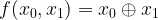
Thus our first task is to develop a quantum equivalent of this function, i.e. a reversible version of f.

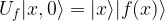
Recall that in general, given a boolean function f, we can define a unitary transformation U_f by the following rule

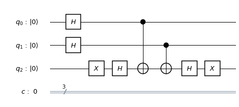
Thus U_f flips the target qubit y if f(x) is one and leaves it unchanged otherwise. In our case, combining this with the definition of the XOR function implies that we are looking for a circuit acting on three qubits – two input qubits and one target qubit – that flips the target qubit if and only if the two input qubits are not equal. From this textual description, it is obvious that this can be constructed using a sequence of two CNOT gates.

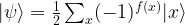
Let us now go through the individual steps of the Deutsch-Jozsa algorithm, using the optimized version published 1997 in this paper by R. Cleve, A. Ekert, C. Macchiavello and M. Mosca (this version is also described in one of my earlier posts but is does not hurt to recap some of that). The first step of the algorithm is to prepare a superposition state

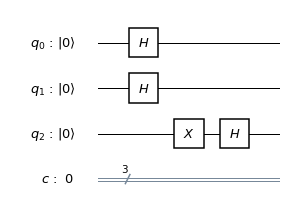
This is accomplished by applying a Hadamard gate to each of the two qubits that make up our primary register in which the variable x lives. We then add an ancilla qubit that is in the state , so that our state is now

So far our circuit looks as follows.

Next we apply the oracle U_f to our state. According to the definition of the oracle, we have

and

Therefore we find that

From this formula, we can read off how U_f acts depending on the value of f(x). If f(x) is 0, the right hand side is equal to the left hand side and U_f acts trivially. If, however, f(x) is one, the right hand side is simply minus the left hand side, and U_f acts as multiplication by -1. Combining this with our previous formula, we obtain

Next, we apply again the Hadamard operator followed by the Pauli X gate to the third qubit (the ancilla), i.e. we uncompute the ancilla qubit. From the expression above, we can read off directly that the result left in the first two qubits will be

This is the vector that we will have in the first two qubits of our quantum register when we have processed the following circuit.

Let us now calculate the overlap, i.e. the scalar product, between this vector and the initial superposition . Clearly,

We find that this overlap is zero if and only if the function f is balanced. But how can we measure this scalar product? To see this, recall that the initial state is the result of applying the tensor product H² of the two Hadamard operators to the first two qubits in the fiducial state. Thus we can write our scalar product as

In other words, we can determine the scalar product by again applying a Hadamard operator to each of the first two qubits and measuring the overlap of the resulting state with the basis state which is the same thing as the probability to measure when we perform a measurement in the computational basis. Thus we finally obtain the following circuit

and the function f is balanced if and only if the probability to measure is zero.

Let us now turn this into Python code using Qiskit. I found it useful to create subroutines that act on a given circuit and build parts of the circuit which can then be tested independently from each other on a simulator before combining them. Here is the code to create the oracle for our balanced function f.

def createOracleBalanced(q,c):
    circuit = QuantumCircuit(q,c)
    circuit.cx(q[0], q[2])
    circuit.cx(q[1], q[2])
    circuit.barrier(q)
    return circuit

Similarly, we can write routines that create the initial state and join the ancilla qubit.

def createInitialState(circuit):
    circuit.h(q[0])
    circuit.h(q[1])
    circuit.barrier(q)

def addAncilla(circuit):
    circuit.x(q[2])
    circuit.h(q[2])
    circuit.barrier(q)

Finally, we need to be able to uncompute the ancilla and to add the final measurements.

def uncomputeAncilla(circuit):
    circuit.h(q[2])
    circuit.x(q[2])
    circuit.barrier(q)

def addMeasurement(circuit):
    circuit.h(q[0])
    circuit.h(q[1])
    circuit.barrier(q)
    circuit.measure(q[0], c[0])
    circuit.measure(q[1], c[1])
    circuit.barrier(q)

A word on barriers. In this example code, we have added barriers after each part of the circuit. Barriers are an element of the OpenQASM specification and instruct the compiler not to combine gates placed on different sides of a barrier during optimization. In Qiskit, barriers have the additional benefit of structuring the visualization of a circuit, and this is the main reason I have included them here. In an optimized version, it would probably be safe to remove them.

After all these preparations, it is now easy to compile the full circuit. This is done by the following code snippet – note that we can apply the + operator to two circuits to tell Qiskit to concatenate the circuits.

q = QuantumRegister(3,"q")
c = ClassicalRegister(3,"c")
circuit = QuantumCircuit(q,c)
createInitialState(circuit)
addAncilla(circuit)
circuit = circuit + (createOracleBalanced(q,c))
uncomputeAncilla(circuit)
addMeasurement(circuit)

We can then compile this code for a simulator or a backend as explained in my last post on the IBM Q experience (you can also find the full source code here). The following histogramm shows the result of the final measurement after running this on the ibmqx4 5 qubit quantum computer.

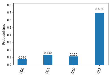
We see, as in the experiments conducted before, that the theoretically expected result (confirmed by running the circuit on a simulator) is blurred by noise – we get the value 00 in a few instances, even though the function is balanced. Even though the outcome can still be derived with a reasonable likelihood, we start to get a feeling for the issues that we might have with noise for more complex functions and circuits.

It is instructive to extract the compiled QASM from the resulting qobj and load that code into the IBM Q Experience composer. After a few beautifications, the resulting code (which you can get here) is displayed as follows in the composer.

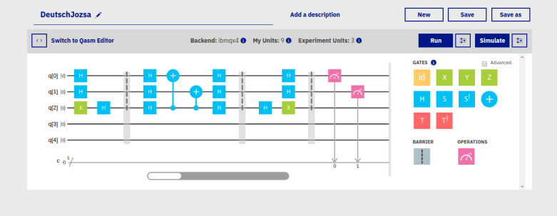
If we compare this to the original circuit, we see that the compiler has in fact rearranged the CNOT gates that make up our oracle. The reason is that the IBMQX4 device can only realize specific CNOT gates. It can, for instance, implement a CNOT gate with q[1] as control as q[0] as target, but not vice versa. Therefore the compiler has added Hadamard gates to swap control and target qubit. We also see that the compiler has respected the barriers and not cancelled some of the double Hadamard gates. If we remove the barriers and remove all Hadamard gates that clearly cancel each other, we finally obtain a greatly simplified version of the circuit which looks as follows.

Of course this simplification hinges on the special choice of the function f. Nevertheless, it is useful – fewer gates mean fewer errors. If we compare the error rates of the optimized circuit with the new circuit, we find that while the original version had an error (i.e. an unexpected amplitude of ) of roughly 10%, a run with the optimized circuit showed an error of only 5,5%.

This completes our post. The next algorithm that we will implement is Shor’s algorithm and the quantum Fourier transform.