In the previous post, we have discussed recurrent neural networks in the context of language processing, but in fact, they can be used to learn any type of data structured as a time series. To make sure that we really understand how this works before proceeding to more complex models, we will spent some time today and teach a simple RNN on a very specific sequence – we will teach it how to count.
As usual, this post comes with a notebook that you can either run locally (please follow the instructions in the README to set up a local environment, no GPU needed for today) or in Google CoLab using this link. So I will not go through all the details in the code, but focus on the less obvious parts of it.
First, let us discuss our dataset. Today we will in fact not ta ckle language related tasks, but simply train a model to predict the next element in a sequence. These elements are numbers between 0 and 127, and the sequences that make up our training data set are simply all sequences of six consecutive numbers in this range, like [3,4,5,6,7,8] or [56,57,58,59,60,61]. The task that the model will learn is to predict the next element in a given sequence. If, for example, we present it the sequence [3,4,5], we expect it to predict that the next element is 6.
So our dataset is really simple, the only actual work that we have to do is to convert our data items into tensors. Our input data will be one-hot encoded, so that a sequence of length L has shape (L,V) where V = 128. Our targets will just be labels, so the targets for a sequence of length L will be L labels, i.e. a tensor of shape L. Here is the code to generate an item in the dataset.
#
# Input at index is the sequence of length L
# starting at index
#
inputs = torch.arange(index, index + self._L, dtype = torch.long)
targets = torch.arange(index + 1, index + self._L + 1, dtype = torch.long)
#
# Convert inputs to one-hot encoding
#
inputs = torch.nn.functional.one_hot(inputs, num_classes = self._V)
inputs = inputs.to(torch.float32)
Next, let us discuss our model. The heart of the model will of course be an RNN. The input dimension will be V, as we plan to present the input as one-hot encoded vectors. We have already seen the forward function of the RNN in the last blog post, and it is not difficult to put this into a class that is a torch.nn.Module. Keep in mind, however, that the weights need to be wrapped into instances of torch.nn.Parameter so that they are detected by the optimizer during learning.
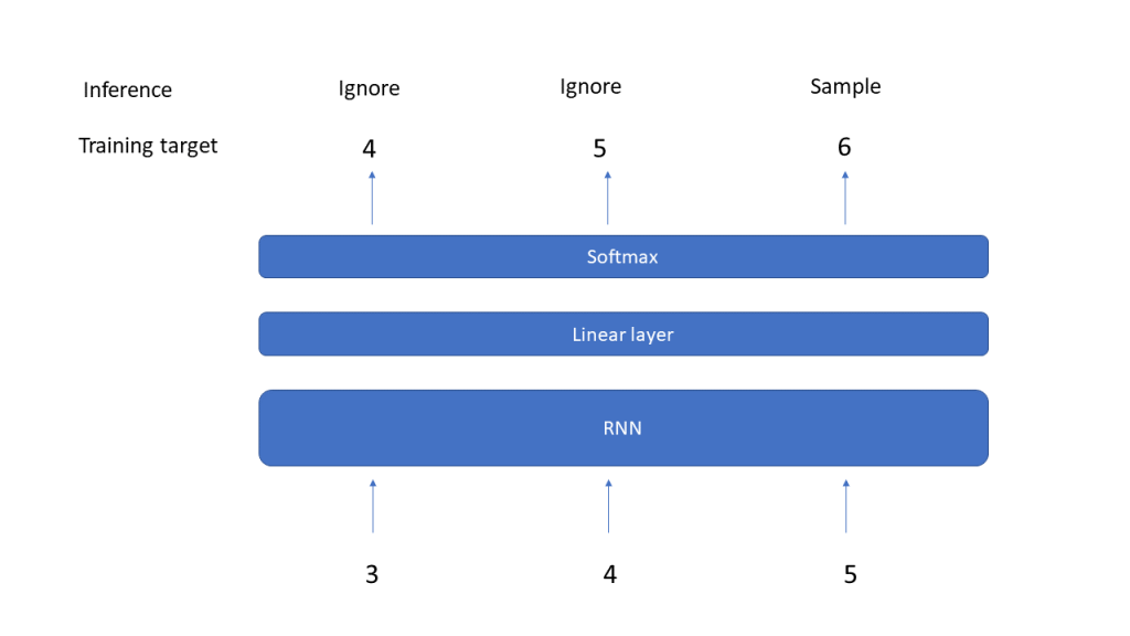
The output of the RNN will be the output of the hidden layer and will be of shape (L,D), where L is the length of the input sequence and D is the inner dimension of the model. To predict the next elements of the sequence from this, we add a linear layer that maps this back into a tensor of shape (L, V). We then take the last element of the output, which is a tensor of shape V, and apply a softmax to get a probability distribution. To make a prediction, we could now either sample according to this multinomial distribution, or just take the element with the highest probability weight – we will discuss more advanced sampling methods in a later post.
So here is the code for our model – note that we again allow a previous hidden layer value to be used as optional input.
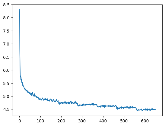
We can now train our model by putting the logic for the generation of samples above into a Torch dataset, firing up a data loader, instantiating a model and going through the usual training procedure. Our data set is sufficiently small to make the model converge quickly (this is of course a massive case of overfitting, but for our purposes this is good enough). I used a hidden dimension of 32 and a batch size corresponding to half of the dataset, so that one epoch involves two gradient updates. Here is a diagram showing the training loss per epoch over time.
Having trained our model, we can now go ahead and make predictions. We have already indicated how this works. To predict the next item of a given sequence, we feed the sequence into the model – note that this sequence can be longer or shorter than those used during training. The output of the model will be a tensor of shape (L, V). We only use the last time step for prediction, apply a softmax to it and pick the element with the highest weight.
#
# Input is the sequence [7,8,9,10]
#
input = torch.arange(7, 11, dtype=torch.long)
print(input)
input = torch.nn.functional.one_hot(input, num_classes = V)
input = input.to(torch.float32)
out, hidden = model(input.to(device))
#
# Output has shape (L, V)
# Strip off last output and apply softmax
# to obtain a probability distribution p of length V
#
p = torch.softmax(out[-1], dim = -1)
#
# Predict
#
guess = torch.argmax(p).item()
print(guess)
If everything worked, the result will be 11, as expected, so our model learns what it is supposed to learn.
There is an important lesson to learn from this simple example. During inference, the output that we actually use is the output of the last time step, i.e. of the last iteration inside the forward method (this is not the case for all tasks on which RNNs are typically trained, but for many of them). At this point, the model has only access to the last input x[t], so that all information about previous time steps that the model needs to make a prediction have to be part of the hidden layer. In that sense, the hidden layer really serves as a memory and helps the model to remember previously seen input in the same sequence.
Of course our example is a bit of an exception, as the model only needs the last value to make the actual prediction. In the next post, we will challenge the model a bit more and ask it to make a prediction that really requires a memory, namely to predict the first element of a sequence, which the model thus needs to remember until the very last element is processed. We will be able to see nicely that this gets more difficult as the sequence length grows and discuss a special type of RNNs called long-short term memory neural networks (LSTM for short) that have been designed to increase the ability of a network to learn long-range dependencies.
When designing neural networks to handle language, one of the central design decisions you have to make is how you model the flow of time. The words in a sentence do not have a random order, but the order in which they appear is central to their meaning and correct grammar. Ignoring this order completely will most likely not allow a network to properly learn the structure of language.
We will later see that the transformer architecture uses a smart approach to incorporate the order of words, but before these architectures were developed, a different of models was commonly used to deal with this challenge – recurrent neural networks (RNNs). The idea of a recurrent neural network is to feed the network one word at a time, but to allow it to maintain a memory of words it has seen, or, more precisely, of their representations. This memory is called the hidden state of the model.
To explain the basic structure of an RNN, let us see how they are used to solve a very specific, but at the same time very fundamental problem – text generation. To generate text with a language model, you typically start with a short piece of text called the prompt and ask the model to generate a next word that makes sense in combination with the prompt. From a mathematical point of view, a word might be a good candidate for a continuation of the prompt if the probability that this word appears after the words in the prompt is high. Thus to build a model that is able to generate language, we train a model on conditional probabilities and, during text generation, choose the next word based on the probabilities that the model spits out. This is what large language models do at the end of the day – they find the most likely continuation of a started sentence or conversation.
Suppose, for instance, that you are using the prompt
“The”
Let us denote this word by w1. We are now asking the model to predict, for every word w in the vocabulary, the conditional probability
that this word appears after the prompt. We then sample a word according to this probability distribution, call it w2 and again calculate all the conditional probabilities
to find the next word in the sentence. We call this w3 and so forth, until we have found a sentence of the desired length.
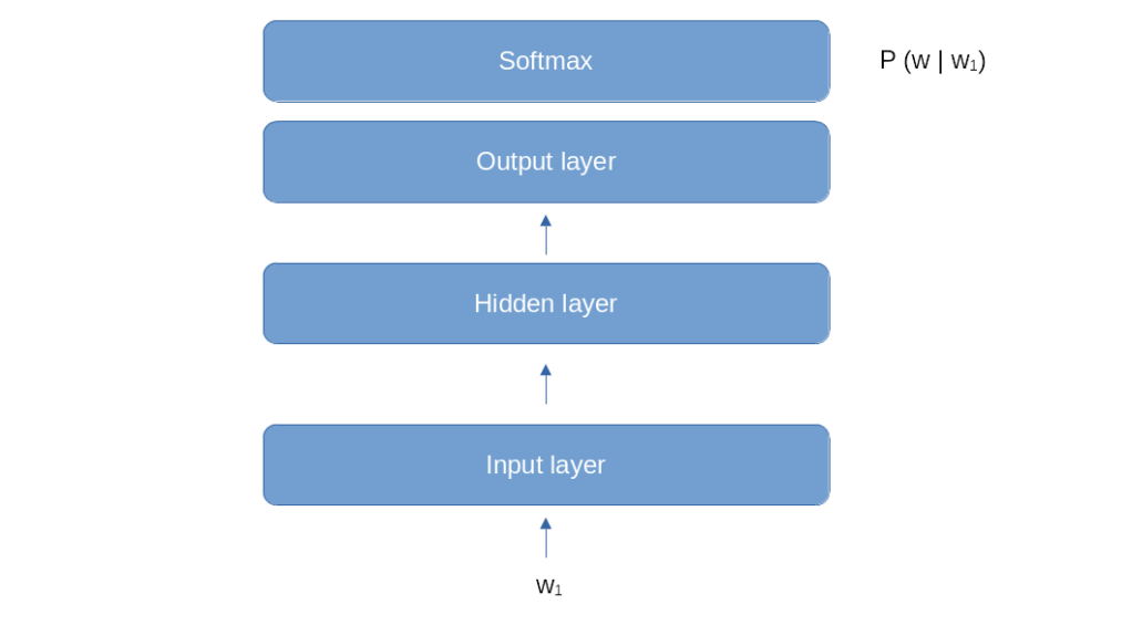
Let us now think about a neural network that we could use for this purpose. One approach could be an architecture similar to the one that we used for word2vec. We start with an embedding, followed by a hidden layer of a certain size (the internal dimension of the model), and add an output layer to convert back into V dimensions, were, as before, V is the size of our vocabulary.
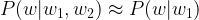
This model looks like a good fit for the first step of the word generation. If our prompt consists of one word w1, and we need to calculate the conditional probabilities P(w | w1), we could do this by feeding w1 into the model and train it to predict the probabilities P(w | w1) in its softmax layer, very much like a classical classification problem. However, things become more difficult if we have already generated two words and therefore need to calculate a conditional probability P(w | w1, w2) that depends on the two previous words. We could of course simply ignore w1 and only feed w2, which amounts to approximating
This, however, is a very crude approximation (sometimes called a unigram model), in general, the next sentence in a word will not only depend on the previous word, but on all previous words. Just think of the two sentences
Dinosaurs are big animals
Mice are small animals
If we wanted to determine the most likely word after “are”, the first word clearly does make a difference. So we need to find a way to make the previous words somehow available to our model. The approach that an RNN (or, more precisely, an Elman RNN) takes is to use a hidden layer which does not only have one input (the output of the lowest layer) but two inputs. One input is the output of the lowest layer, and the second input is the output of the hidden layer during the previous time step.
Let us go through this one by one. First, we feed word w1 into the model as before. This goes through the input layer, through the hidden layer and finally through the output layer. However, this time, we save the output of the hidden layer and call it h1. In the second step, we feed w2 into the model. Again, this goes through the input layer. But now, we combine the value of the input layer with our previously saved h1 and feed this combined value into the hidden layer to get an output h2. We again save this, but also feed it into the output layer. In the next step, we read word w3, combine the result of the input layer with h2, feed this into the hidden layer and so forth. So at step t, the input the hidden layer is a function of ht-1 (the value of the hidden layer in the previous step) and it (the value of the input layer at time t).
I actually found it difficult to understand this when I first read about RNNs, but sometimes code can help. So let us code this in Python. But before we do this, we need to make it more precise what it means to “combine” the value of the hidden layer from the previous time step with the value of the input layer. Combination here means essentially concatenation. More precisely, we have two weight matrices that determine the value of the hidden layer. The first matrix that we will call Wih (the indices mean input-to-hidden) is applied to the inputs. The second one that we will call Whh (hidden-hidden) is applied to the value of the hidden layer from the previous time step. Taking activation functions and bias into account, the value of the hidden layer at time t is therefore
where xt is the input at time t. Note how the output from the previous step ht-1 sneaks into this equation and realizes the feedback loop indicated in the diagram above.
Armed with this understanding, let us implement a simple RNN forward method that accepts L words (or, more generally, input vectors) and applies the above processing steps, i.e. processes L time steps.
 def forward(x):
    L = x.shape[0]
    h = torch.zeros(d_hidden)
    out = []
    for t in range(L):
        h = torch.tanh(x[t] @ w_ih.t() + b_ih + h @ w_hh.t() + b_hh)
        out.append(h)
    return torch.stack(out)
Here, d_hidden is the dimension of the hidden layer. Note that we not not include the output layer which is actually common practice (the RNN model class that comes with PyTorch does not do this either). We can clearly see that the hidden state h is saved between the individual time steps and can therefore help the model to remember information between time steps, for instance some features of the previous words that are helpful to determine the next word in the sequence.
The output of our forward function has shape (L, d_hidden), so that we have one hidden vector for every time step. We could feed this into an output layer, followed for instance by a softmax layer. Typically, however, we are only interested in the output of the last time step, which we would interpret as the conditional probability for the next word as discussed above.
Unfortunately, our forward function still has a problem. Suppose we start with a prompt with L = 3 words. We encode the words, call the forward function and obtain an output. We take the last element of the output, feed it into a feed forward layer to map back into the vocabulary, apply softmax and sample to get the next word. When we now want to determine the next word, however we would have to repeat the same procedure for the first three words to get our hidden state back that we need for the last time step. To avoid this, it would be useful if we could pass a previous hidden state as optional parameter into our model so that the forward function can pick up where it left. Similarly, we want our forward function to return the hidden layer value at the last time step as well to be able to feed it back with the next call. Here is our modified forward function.
def forward(x, h = None):
    L = x.shape[0]
    if h is None:
        h = torch.zeros(d_hidden)
    out = []
    for t in range(L):
        h = torch.tanh(x[t] @ w_ih.t() + b_ih + h @ w_hh.t() + b_hh)
        out.append(h)
    return torch.stack(out), h
This looks simple enough, but it is actually a working RNN. It is instructive to compare the output that this simple forward function produces with the output of PyTorchs torch.nn.RNN module. The GitHub repository for this series contains a simple notebook doing this, which you can again either run locally (no GPU needed) or in Google Colab using this link. This notebook also shows how to extract the weight and bias vectors from an RNN in PyTorch.
We have not yet explained how an RNN is trained. Suppose again we wanted to train an RNN for text generation. We would then pick a large corpus of text as a training dataset to obtain a large number of sentences. Each sentence would create a training sample. To force the model to predict the next word, the targets that we use to calculate the loss function are obtained by shifting the input sequence by one position to the right. If, for instance, our dataset contains the sentence “I love my cute dog”, we would turn this into a pair of inputs and targets as follows.
In particular, the target label does not depend on the prediction that the model makes during training, but only on the actual data (the “ground truth”). If, for instance, we feed the first word “I” and the model does not predict “love” but something else, we would still continue use the label “my,”, even if this does not make sense in combination with the actual model output.
This method of training is often called teacher forcing. The nice thing about this approach is that it does not require any labeled data, i.e. this is a form of unsupervised learning. The only data that we need is a large number of sentences to learn the probabilities, which we can try to harvest from public data available on the internet, like Wikipedia, social media or projects like Project Gutenberg that make novels freely available. We will actually follow this approach in a later post to train an RNN on a novel.
This concludes our post for today. In the next post, we will make all this much more concrete by implementing a toy model. This model will learn a very simple sequence, in fact we will teach the model to count, which will allow us to demonstrate the full cycle of implementing an RNN, training it using teacher forcing and sampling from it to get some results.
In the last post, we have looked at how a text is pre-processed to make it accessible for a neural network and have seen that the first step is to convert a text into a sequence of numbers, where each number is the index of the corresponding word in a vocabulary. Let us now discuss how we can convert each of these numbers into a vector.
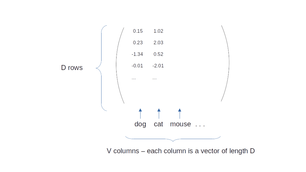
Most machine learning models which are used for natural language processing have a property called the model dimension which we will abbreviate by D. A model dimension of, say, 768, simply means that internally, all words are represented by vectors in a vector space of dimension 768. Thus, a single word is a one-dimensional tensor of length D = 768. Our task is therefore to assign to each word in a vocabulary of size V a vector in a D-dimensional space. This assignment, called the embedding, can be nicely represented as a matrix of dimension D x V, so that the column at position i represents the word with index i in the vocabulary.
Of course there are endless possibilities to construct such an embedding. In most cases, the embedding is a learned parameter, i.e. we start training with a randomly initialized embedding and then apply gradient descent to the embedding matrix as to any other parameter during learning. However, it has become increasingly popular to use an embedding which has already been pre-trained so that training does not start from zero and the model hopefully converges faster. One method that facilitates such a pre-training is called the word2vec algorithm.
The idea of the word2vec algorithm (and of many other approaches to constructing embeddings) is to start with a larger model that contains the embedding we wish to train and a second model part that is adapted to a certain downstream task. We then train the entire model on this downstream task, hoping that the embedding layer will capture not only the specific information required for the downstream task, but more general patterns that are useful for other tasks as well. We then throw away the upper part of the model and reuse the embedding layer for other tasks.
The diagram above shows this architecture. The model consists of an embedding layer which translates a word represented by an index between 0 and V – 1 into a vector of dimension D, the internal model dimension. You can think of this as the combination of a one-hot encoding that turns the index into a vector of dimension V and a linear layer without bias that projects onto D dimensions. This part of the model is, once trained, the actual artefact that we might reuse in other, more complex models.
The upper part of the model is adapted to the specific downstream task on which word2vec has been trained. The original paper actually explains two downstream tasks called CBOW and Skipgram, we will focus on CBOW in this post.
Before describing CBOW, let us first try to explain the underlying objective of the training. We want to construct embeddings that capture not only a word itself, but the meaning of a word. Put differently, we want words that have a similar meaning to end up as nearby vectors. To make this precise, we have to define a notion of similarity for our embeddings, i.e. for D-dimensional vectors, and for words.
For vectors, this is easy. In two-dimensional linear algebra, we would call two vectors similar if they point roughly in the same direction, i.e. if the angle between them is small, or in other words if the cosine of the angle is close to one. There is no good notion of an angle in D-dimensional space, but there is a good replacement for the cosine, namely the dot product. So to measure the similary of two vectors x and y, we can take the normed dot product and simply define this to be the cosine
Defining similarity between words is a bit more complicated. The approach that word2vec takes is to assume that two words have a similar meaning if they tend to appear in the same context, i.e. surrounded by similar sets of words.
To explain this, let us consider a simple sentence (I did not make this up, this sentence actually appears almost verbatim in the training data that we will use later).
“A team of 24 players was selected from an initial pool of 49 candidates”
Let us pick a word in this sentence, say “from”. We can then define the context of this center word to be the set of all words in the sentence that appear within in certain range around the center word. For example if we choose a window size of four, the region that makes up the context extends by two words to the left and two words to the right of the center word. Thus, the context words for the center word “from” are
“was”, “selected”, “an”, “initial”
So the context of a center word is simply the set of all words in the window around the center without the center word itself. The idea of word2vec is that the meaning of a word can be captured by the context words that appear in combination with it. If two center words appear most of the time surrounded by the same context words, then they are considered to have a similar meaning.
To see that this makes sense, consider another example – the sentence “The mighty king is sitting on a golden throne”. If we replace king by “ruler”, the resulting sentence would still be likely to appear in a large corpus of text. As the words “king” and “ruler” can replace each other in their respective context while still making sense, we would consider them to have a similar meaning.
To turn this idea into a training objective, the CBOW algorithm proceeds as follows. First, we go through our data and for each center word, we determine the context as above. Each pair of center word and context will constitute one training sample. We now train the model to predict the center word from the given context. More specifically, we first turn the context into a single vector by feeding each context word into the embedding layer and taking the average of the resulting vectors (this is why the model is called CBOW which is the abbreviation for “continuous bag of words”, as taking the average ignores the position of the word in the context). We now have a single vector of dimension D which we can use as input for a second linear layer which turns it back into a vector of dimension V. This vector is then the input for a softmax so that we eventually obtain an index in the range between 0 and V – 1. The target is our center word and we can apply the usual cross entropy loss function. So CBOW is essentially a classification problem in which the label is the center word and the input is the averaged context.
Note that both the embedding layer and the linear layer do not have a bias, so that they are fully determined by their weight matrices, say U and V. The function to which we apply the softmax is then essentially the matrix product of U with the transpose of V. This in turn is the dot product of the rows of U and the rows of V, which we can both interpret as embeddings. If we write this out in terms of scalar products, you see the cosines emerging and develop an intuition why this training objective does indeed foster the learning of similarities. But instead of diving deeper into this, let us go ahead and discuss the implementation in PyTorch.
To implement the embedding layer without having to make the one-hot encoding explicit, we can use the torch.nn.Embedding class provided by PyTorch. The forward method of this module accepts an index or a sequence of indices and returns a vector or a sequence of vectors, which is exactly what we need. The output layer is an ordinary linear layer. Following the usual practice, we do not add the final softmax layer to our model but use the cross entropy loss function which includes the calculation of the softmax. With this, our model is rather simple:
EMBED_MAX_NORM = 1

class CBOW(torch.nn.Module):

    def __init__(self, model_dim, V, bias = False):
        super().__init__()
        self.embedding = torch.nn.Embedding(
            num_embeddings=V,
            embedding_dim=model_dim,
            max_norm=EMBED_MAX_NORM,
        )
        self.linear = torch.nn.Linear(
            in_features=model_dim,
            out_features=V,
            bias = bias
        )


    def forward(self, Y):
        E = self.embedding(Y).mean(axis=1)
        U = self.linear(E)
        return U
Note the max_norm parameter which re-normalizes the embeddings if they exceed a certain size. Setting this parameter turns out to be helpful during training (a fact that I discovered after reading this excellent blog post by O. Chernytska which turned out to be a very valuable resource when training my model).
We see that the forward method does what we have sketched earlier – we first apply the embeddings which will give us a tensor of shape (B, W, D) where B is the batch size, W is the window size and D is the model dimension. We then take the mean along the middle dimension, i.e. the mean of embedding of all words in the context, which will give us a tensor of shape (B, D). We then apply the output layer to get a batch of shape (B, V) which we use as input to our loss function.
Let us now discuss our data and the preprocessing. To train our model, we will use the WikiText2 dataset which consists of roughly 2 million token taken from Wikipedia and is available via the Torchtext library. Each item in the dataset is a paragraph. Some paragraphs consist of a title only which we remove. We then apply a tokenizer to the remaining paragraphs and collect them in one large list, in which each item is again a list of token.
ds = torchtext.datasets.WikiText2(split="train")
tokenizer = torchtext.data.utils.get_tokenizer("basic_english")
paragraphs = []
for item in ds:
    # Remove trailing whitespace and special characters
    item = re.sub("^\s+", "", item)
    item = re.sub("@", "", item)
    if not re.match("^=", item):
        p = tokenizer(item)
        if len(p):
            paragraphs.append(p)
Next, we build a vocabulary using again the torchtext library. We add a special token “<unk>” to the vocabulary that stands for an unknown word (and is in fact already present in the input data). We also only add token to the vocabulary which appear more than a given number of times, i.e. have a certain minimum frequency.
We can then encode the paragraphs as usual using our vocabulary. Next, we need to create pairs of center word and context out of our training data. Here, it is helpful that we maintain the paragraph structure, as a context that spans across a paragraph is probably less useful, so we want to avoid this. One way to generate the center/context pairs is using a Python generator function, like this.
def yield_context(paragraphs, window_size = 8):
    for p in paragraphs:
        half = window_size // 2
        #
        # If we are not yet at the last token in the paragraph,
        # yield window and advance center.
        #
        for index, center in  enumerate(p):
            context = p[max(0, index - half):index]
            context.extend(p[index + 1:min(len(p), index + half + 1)])
            yield center, context
Here we visit each position in each paragraph and use it as center position. We then carve out half of the window size to the left of the center token and half of the window size to the right and concatenate the result lists, which we return along with the center.
To train our model, we can put all this code into a PyTorch dataset so that we can use it along with a PyTorch data loader. Training is now straightforward. I have used an initial learning rate of 0.1 for a model dimension of 300 and a batch size of 20000. I apply a linear rate scheduler and use an Adam optimizer.
To make it a bit easier for you to try this out, I put together all the code in a notebook that is available in the GitHub repository for this series. To run this, you have several options. First, you can run it locally (or in your favorite cloud environment, of course) by cloning the repository and following the instructions in the README, i.e.
Then navigate to the notebook in the word2vec directory and run it. Alternatively, you can run it in Google Colab by simply clicking on this link. Note that the second cell will install the portalocker package if not yet present, so you might have to restart the runtime afterwards to make sure that the package can be used (use Runtime – restart and run all if you get an error in the third cell saying that portalocker cannot be found).
With the chosen parameters, training is rather smooth and takes less than 10 epochs to achieve reasonable results. In the notebook, I train for 7 epochs to achieve a mean training loss of a bit more than 4.5 in the last epoch (to keep things simple, I do not measure the validation loss).
Once we have trained the model, we can check that it does what we are up to – making sure that similar words or semantically related words receive similar embeddings. To verify this, let us pick a word that appears in the vocabulary and try to find those words in the vocabulary that are closest to it, i.e. have the largest cosines. To do this, we can extract the weights (which PyTorch stores internally with shape (V, D) so that the rows are the embeddings) using the attribute weight of torch.nn.Embedding. Given the embedding of a fixed token, we now need to take the dot product of all rows of the weight matrix with the vector representing the fixed token, which can be conveniently organized as a matrix multiplication. We can then sort the resulting vector and extract the five largest entries. Here is a short piece of code doing this.
 def print_most_similar(token, embeddings, vocab):
    #
    # Normalize embeddings
    #
    _embeddings = torch.nn.functional.normalize(embeddings, dim = 1)
    #
    # get u, the embedding of our token
    #
    u = _embeddings[vocab[token], :]
    #
    # do dot products as one large matrix multiplication
    #
    v = torch.matmul(_embeddings, u)
    #
    # Sort this
    #
    values, indices = torch.sort(v, descending=True)
    print(f"Most similar token for {token}")
    for i in range(5):
        print(f"      {vocab.lookup_token(indices[i])} -- {values[i]}")
If we run this after training for the word “king”, the results we get (which are to some extent random, so you might get slightly different results if you run this yourself) are
king -- 0.9999999403953552
son -- 0.5954159498214722
earl -- 0.59091717004776
archbishop -- 0.57264244556427
pope -- 0.5617164969444275
This is not bad for two minutes of training! Except the second one, all others are clearly some sort of ruler and in that sense will probably appear in similar semantic roles as the word “king”.
There is one more experiment that we can make. Remember that the second layer of our model converts the vectors from the internal dimension back into the vocabulary. This is a linear layer with a weight matrix that has the same shape as that of the embedding! Thus we actually learn two embeddings – the embeddings that we have modelled as a torch.nn.Embedding layer and that we apply to the context vectors (the context embedding) and the embedding that is implicit in the linear layer of type torch.nn.Linear that one might call the center embedding. We can repeat the test above with the center embedding (again, look at the notebook for the details) and get a very similar output.
 king -- 1.0
 pope -- 0.6784377694129944
 lord -- 0.6100903749465942
 henry -- 0.5989689230918884
 queen -- 0.5779016017913818
With this, let us close this post for today. If you want to read more on word2vec, the Skipgram mechanism that we have not presented and more advanced versions of the algorithm, I have listed a few valuable reads below. In this series, we will continue with an introduction to RNNs, a generation of network architectures that are important to understand as many training methods and terms used for transformers as well go back to them.
In the history of AI, progress has always come from several sources – more powerful hardware, more high-quality training data or refined training methods. And sometimes, we have seen a step change triggered by a new and innovative generation of models.
Some of you might remember the time when the term Deep Learning was coined, referring to machine learning models consisting of several stacked layers of neural networks. Later, convolutional neural networks (CNNs) took computer vision and image recognition by storm, and recurrent neural networks and in particular LSTMs where widely applied to boost applications in natural language processing like machine translation or sentiment analysis.
Similarly, the recent revolution in natural language processing has been triggered by a novel type of neural networks called Transformers which is very well adapted to the specific challenges of processing long sentences. In fact, all of the currently hyped language models like GPT , Googles LaMDA or Facebooks LLaMA are based on the transformer architecture – so clearly that is something that everybody interested in machine learning should probably understand.
This is what we will do in this series – take a deeper look at the transformer architecture, understand how these models are implemented and trained and learn how pre-trained, publicly available models can easily be downloaded and used. We will cover both the theory, referring to the original papers on the subject if that makes senses, and practice, using the PyTorch framework to implement some networks and training scripts ourselves.
More specifically, we will cover the following topics in this series:
the basics of NLP – tokenization, vocabularies and language modelling tasks
Obviously, we cannot start from zero to be able to cover all this. So I assume some familiarity with machine learning and neural networks (if this is new to you, you might want to read some of the excellent available introductions like chapter 7 of Speech and Language processing by Jurafsky and Martin, which also covers parts of what we will discuss, chapter 3 and 4 of Dive into Deep Learning or chapter 5 – 7 of Machine learning with neural networks by B. Mehlig). I also assume that you understand the basics of PyTorch, if not, I recommend the excellent introduction to PyTorch which is part of the official documentation.
Tokenization, vocabularies and basis tasks in NLP
After this short outlook of what’s ahead, let us dive right into the content. We start by explaining some terms that you will see over and over again if you get into the field of natural language processing (NLP).
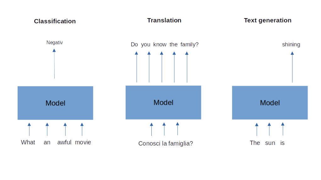
First, let us discuss some of the common problems that NLP tries to solve. Some of these problems can be described as a classification task. The input that machine learning models receive is a text, consisting of a sequence of words or, more generally, token (we get to this in a minute), and the output is a label. An example for this type of task is sentiment analysis. The model is given a text, for instance a review of a movie or a book, and is asked to predict whether the overall sentiment of the review is positive or negative. Note that the input to the model, the text, has a linear structure – each word has a position, so there is a notion of time in the input – while the output is simply a label.
A second class of tasks is sometimes called sequence-to-sequence and consists of receiving a sequence of words as an input and providing a sequence of words as output. The prime example is machine translation, which receives a sequence of words in the source language as input and produces a translation into the target language. Note that the length of the target and length of the source are, in general, different.
Finally, a third class of problems (there are many more in NLP) that we will be concerned with is text generation. Here the task is to create a text which appears natural and fluent (and of course grammatically correct) from scratch, maybe be completing a short piece of text fed into the model called the prompt. We will see later that machine translation can actually be expressed as conditional text generation, i.e. text generation giving some context which, in the case of a translation task will be an encoding of the input sequence.
For all of these tasks, we will have to find a reasonable way to encode a sequence of words as number or, more precisely, as vectors. Typically, this proceeds in several steps. The first step is tokenization which means that we break down our text into a list of tokens. Initially, a token will be a word or a punctuation character, but later we will turn to more general tokens which can be parts of words or even individual characters. The most straightforward way to do this is to split a text along spaces, i.e. to do something like
text = "My name is John. What is your name?"
token = text.split()
print(token)
This is simple, maybe too simple. We combine, for instance, a punctuation mark along with the word after which it follows, which might not be a good idea as a punctuation mark has an independent syntactical meaning. We also do not convert our words to lower- or uppercase, so that “Name” and “name” would be different token. There are many ready-to-use implementations of more sophisticated approaches. For now, we will use the tokenizer that is part of the Torchtext library. To use this, please make sure that you have torch and torchtext installed, I have used version 2.0.0 of PyTorch and version 0.15.1 of Torchtext, but older versions should work as well. We can than tokenize the same text as before as follows.
We see that the tokenizer has converted all words into lower-case and has translated punctuation marks into individual token.
The next stage consists of building a list of all known token that appear in our text, i.e. of all unique token. This can conveniently be done using a counter. Here is a short code snippet that creates a list of all unique token.
import collections
token = tokenizer(text)
counter = collections.Counter(token)
vocabulary = [t for t in counter.keys()]
print(vocabulary)
# Output: ['my', 'name', 'is', 'john', '.', 'what', 'your', '?']
So far, our token are still words. To feed them into a neural network, we will have to encode them as numbers. For that purpose, we replace each token in the original text by its index in the vocabulary, so that the initial text is turned into a sequence of numbers. Note that this sequence still preserves the sequential structure, i.e. the order of numbers is the same as the order of the corresponding words in the original sentence (there are other models, commonly referred to as bag-of-word models, in which only the unordered set of token is considered).
stois = dict()
for idx, t in enumerate(vocabulary):
    stois[t] = idx
encoded_text = [stois[t] for t in token]
print(encoded_text)
# Output: [0, 1, 2, 3, 4, 5, 2, 6, 1, 7]
Of course, we can revert this process by replacing each index in the list by the corresponding token, a process known as decoding.
decoded_text = " ".join([vocabulary[idx] for idx in encoded_text])
print(decoded_text)
# Output: my name is john . what is your name ?
Most tokenizers will, in addition to the token generated by identifying words in the text, use additional special token that represent of instance unknown words (i.e. words which are not in the vocabulary as they have not been part of the text used to build the vocabulary) or the end or beginning of a sentence.
At this point, we have converted text into a sequence of numbers. In order to be meaningful as input to a neural network, we now have to turn each of these numbers into a vector. A straightforward approach would be to use one-hot encoding. Suppose that our vocabulary has V items. Then we can turn an index i into a vector in V-dimensional space which is one at position i and zero at all other positions. In other words, the encodings form a base of the vector space on which the model will then operate. This encoding is simply, but has two major drawbacks. First, it treats all words in the same way, regardless of their meaning. It would be nice to have an embedding that translates words into vectors in such a way that similar words end up as somehow similar vectors. Second, the vector space become huge. A vocabulary can easily be as big as 50 k or more token, so our vector space would have 50.000 dimensions, blowing up the model unnecessarily. For those reasons, other procedures to turn words into vectors are more common, which will be the topic of the next post. If you want to try out what we have discussed today, you can download a notebook here and play with it.