The quantum Fourier Transform

We are getting closer to the most spectacular early quantum algorithm – Shor’s algorithm for factoring large composite numbers which can be used to break the most widely used public key cryptography systems. But before we can tackle this algorithm, there is one more thing that we need to understand – the quantum Fourier transform.

The discrete Fourier transform

Let us leave the quantum world for a few moments and take a look at a classical area in mathematics – the discrete Fourier transform. To motivate the definition to come, let us for a moment assume that we are observing a time dependent signal, i.e. a function f(t) depending on the time t. Let us also assume that we are interested in processing this signal further, using a digital computer. This will force us to reduce the full signal to a finite number of values, i.e. to a set of values f(0), f(1), …, f(N-1) at N discrete points in time.

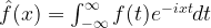
Now assume that we wanted to calculate the classical Fourier transform of this function, i.e. the function $\hat{f}$ given by (the exact formula depends on a few conventions)

$\hat{f}(x) = \int_{-\infty}^{\infty} f(t) e^{-i x t} dt$

If we now replace the function f by the sum of those functions which have value f(i) over a range of length 1, i.e. by its discrete version, this formula turns into

$\hat{f}(x) = \sum_{t=0}^{N-1} f(t) e^{-i x t}$

Now we could code the discrete values f(0), f(1), .. as a sequence x_k of numbers, and we could apply the same process to the Fourier transform and replace it by a sequence X_k of numbers, representing again the values at the discrete points 0, 1, …. The above formula then tells us that these numbers would be given by

$X_k = \sum_{j=0}^{N-1} x_j e^{-i j k}$

We could now look at this formula as giving us an abstract mapping from the set of sequences of N numbers to itself, provided by (putting in a factor $2 \pi / N$ )

$X_k = \sum_{j=0}^{N-1} x_j e^{- \frac{2\pi i}{N} j k}$

This transformation is called the discrete Fourier transform.

There is a different way to look at this which is useful to derive some of the properties of the discrete Fourier transform. For every k, we can build the N-dimensional complex vector $u^k$ with components $u^k_n$ by setting

$u^k_n = e^{\frac{2\pi i}{N} k n}$

These vectors are mutually orthogonal with respect to the standard hermitian product. In fact, the product of any two of these vectors is given by

$(u^k u^{k'})^* = \sum_{j=0}^{N-1} e^{\frac{2\pi i}{N}j(k-k')}$

If $k = k'$ , this is clearly N. Otherwise, we can write this as

$(u^k u^{k'})^* = \sum_{j=0}^{N-1} q^j$

with

$q=e^{\frac{2\pi i}{N}(k-k')}$

If q is not equal to one, i.e. if k is not equal to k’, then, according to the usual formula for a geometric series, this is equal to

$\frac{1-q^{N}}{1-q}$

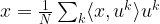
However, this is zero, because $q^N = 1$ due to the periodicity of the exponential function.

Using this orthogonal basis, we can write the formula for the discrete Fourier transform simply as the hermitian product

$X_k = \langle x, u^k \rangle$

In particular, the discrete Fourier transform can be seen as the linear transformation that maps the k-th unit vector onto the vector $(u^k)^*$ . By adding a factor $1 / \sqrt{N}$ , this can be turned into a unitary transformation, i.e. in a certain sense the discrete Fourier transform is simply a rotation. This relation can also be used to easily derive a formula for the inverse of the discrete Fourier transform. In fact, if we expand the vector x into the basis $\{u^k\}_k$ , we obtain

$x = \frac{1}{N} \sum_k \langle x, u^k \rangle u^k$

and therefore

$x_k = \langle x, e_k \rangle = \frac{1}{N} \sum_j \langle x, u^j \rangle \langle u^j, e_k \rangle = \frac{1}{N} \sum_j X_j e^{\frac{2\pi i}{N} jk}$

Fourier transforms of a periodic sequence

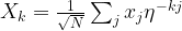
For what follows, let us adapt and simplify our notation a bit. First, we add a factor $1 / \sqrt{N}$ to the formula for the Fourier coefficient, so that the Fourier transform is unitary. Second, we use the symbol $\eta$ to denote the N-th root of unity, i.e.

$\eta = e^{\frac{2\pi i }{N}}$

With this notation, the formula for the Fourier coefficient is then

$X_k = \frac{1}{\sqrt{N}} \sum_j x_j \eta^{-kj}$

and the inverse is given by

$x_k = \frac{1}{\sqrt{N}} \sum_j X_j \eta^{kj}$

Let us now study a special case that is highly relevant for the applications to the factoring of large numbers – the Fourier transform of a periodic sequence. Thus, suppose there is a sequence x_k and a number r called the period such that

$x_{rs + t} = x_t$

for all values of s and t that lead to valid indices. Thus, roughly speaking, after r indices, the values of the sequence repeat themselves. It is also common to reserve the term period for the smallest number with this property. We call the number $u = \frac{N}{r}$ the frequency of the sequence.

Let us now assume that the frequency is a natural number, i.e. that the period divides N, and let us try to understand what this means for the Fourier transform. Using the periodicity, we can write the coefficients as follows.

$X_k = \frac{1}{\sqrt{N}} \sum_j x_j \eta^{-jk} = \frac{1}{\sqrt{N}} \sum_{s,t} x_{sr + t}\eta^{(-sr+t)k} = \frac{1}{\sqrt{N}} (\sum_s \eta^{-srk})(\sum_t x_t \eta^{-tk})$

where s runs from 0 to u-1. We can now write the first of the sums as follows.

$\sum_{s=0}^{u-1} \eta^{-srk} = \sum_{s=0}^{u-1} e^{-\frac{2\pi i}{u}s k}$

Now this is again a geometric series with $q = e^{-\frac{2\pi i}{u}k}$ ! We can therefore conclude as above that this is zero unless q is one, i.e. unless k is a multiple of the frequency u. Thus we have shown that if the sequence x_k is periodic with integral frequency u, then all Fourier coefficients X_k are zero for which k is not a multiple of the frequency.

In the later applications, this fact will be applied in a situation where we know that a sequence is periodic, but the period is unknown. We will then perform a Fourier transformation and inspect the coefficients X_k. We can then conclude that the unknown frequency u must be a common divisor of all those indices k for which X_k is different from zero. This is exactly true if the period divides N, and we will see later that in important cases, it is still approximately true if the period does not divide N.

A quantum algorithm to compute the discrete Fourier transform

Let us now carry over our considerations to the world of quantum computing. In a quantum computer with n qubits, the Hilbert space of states is N-dimensional with N=2ⁿ, and is spanned by the basis $|k \rangle$ . Every vector can be described by the sequence of its coefficients when expanding it into this basis. Consequently, the discrete Fourier transform defines a unitary transformation on the Hilbert by applying the mapping

$\sum_k x_k |k \rangle \mapsto \sum_k X_k |k \rangle$

Now this is a unitary transformation, and as any such transformation, can be implemented by a quantum circuit. We will not go into details on this, see for instance [1], section 7.8 or section 5.1 of [2] (but be careful, these authors use a different sign convention for the Fourier transform). The important part, however, is that a quantum Fourier transform for N=2ⁿ can be realized with O(n²) quantum gates.

In contrast to this, the best known classical algorithms for computing the discrete Fourier transform are commonly known as fast Fourier transform and require O(Nn) steps. Thus it seems that we have again found a quantum algorithm which is substantially faster than its classical counterpart.

Unfortunately, this is not really true, as we have not yet defined our measurement procedure. In fact, if we measure the result of applying a quantum Fourier transform, we destroy the superposition. In addition, the coefficients in which we are interested are the amplitudes of the possible outcomes, and there is no obvious way to measure them – even if we perform the transformation several times and measure over and over again, we only obtain approximations to the probabilities which are the absolute values of the squared amplitudes, so we do not obtain the phase information. Therefore, it is far from clear whether a quantum algorithm can help to compute the Fourier transform more efficiently than it is possible with a classical algorithm.

However, most applications of the Fourier transform in quantum algorithms are indirect, using the transform as a sort of amplification step to focus amplitudes on interesting states. In the next post, we will look at Shor’s algorithm with exploits the periodicity properties of the Fourier transform to factor large composite numbers.

References

1. E. Rieffel, W. Polak, Quantum computing: a gentle introduction, MIT Press
2. M.A. Nielsen, I.L. Chuang, Quantum computation and quantum information, Cambridge University Press

The quantum Fourier Transform

The discrete Fourier transform

Fourier transforms of a periodic sequence

A quantum algorithm to compute the discrete Fourier transform

References

Published by christianb93

2 Comments

Leave a Comment Cancel reply

The discrete Fourier transform

Fourier transforms of a periodic sequence

A quantum algorithm to compute the discrete Fourier transform

References

Share this:

Like this:

Related

Published by christianb93

2 Comments

Leave a Comment Cancel reply