May 2020 – LeftAsExercise

Learning Kafka with Python – installation

In this post, we will install a Kafka cluster with three nodes on our lab PC, using KVM, Vagrant and Ansible.

The setup

Of course it is possible (and actually easy, see the instructions in the quickstart section of the excellent Apache Kafka documentation) to run Kafka as a single-node cluster on your PC. The standard distribution of Kafka contains all you need for this, even an embedded ZooKeeper and a default configuration that should work out-of-the-box. Some of the more advanced topics that we want to try it in the course of this series, like replication and failover scenarios, do however only make sense if you have a clustered setup.

Fortunately, creating such a setup is comparatively easy using KVM virtual machines and tools like Vagrant and Ansible. If you have never used these tools before – do not worry, I will show you in the last section of this post how to download and run my samples. Still, you might want to take a look at some of the previous posts that I have written to get a basic understanding of Ansible and Vagrant with libvirt.

In our test setup, we will be creating three virtual machines, each sized with two vCPUs and 2 GB of memory. On each of the three nodes, we will be running a ZooKeeper instance and a Kafka broker. Note that in a real-world setup, you would probably use dedicated nodes for the ZooKeeper ensemble, but we co-locate these components to keep the number of involved virtual machines reasonable.

Our machines will be KVM machines running Debian Buster. I have chosen this distribution primarily because it is small (less than 300 MB download for the libvirt vagrant box) and boots up blazingly fast – once the initial has initially been downloaded to your machine, creating the machines from scratch takes only a bit less than a minute.

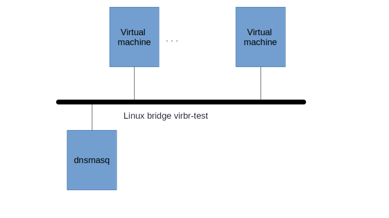
To simulate a more realistic setup, each machine has two network interfaces. One interface is the default interface that Vagrant will attach to a “public” network and that we will use to SSH into the machine. On this interface, we will expose a Kafka listener secured using TLS, and the network will be connected to the internet using NATing. A second interface will connect to a “private” network (which, however, will still be reachable from the lab PC). On this network, we will run an unsecured listener and Kafka will use this interface for inter-broker communication and connecting to the ZooKeeper instances.

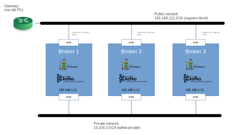
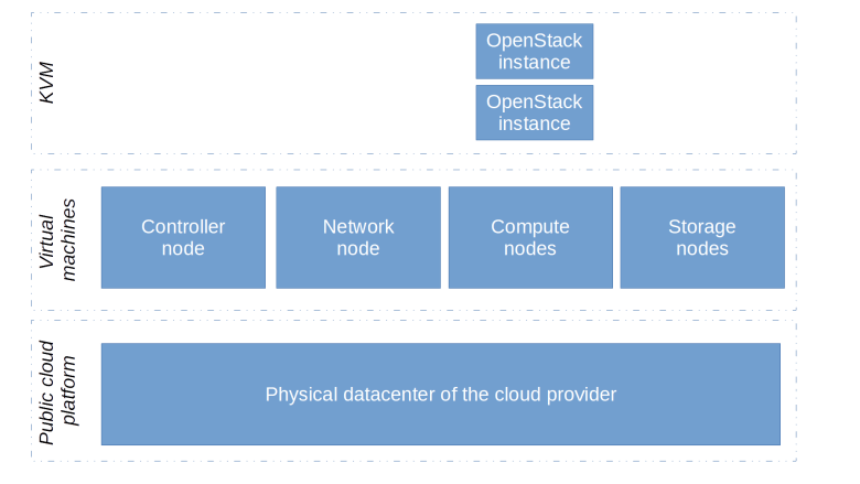
Using the public interface, we will be able to connect to the Kafka brokers via the TLS secured listener and run our sample programs. This setup could easily be migrated to your favored public cloud provider.

Installation steps

The installation is mostly straightforward. First, we setup networking on each machine, i.e. we bring up the interfaces, assign IP addresses and add the host names to /etc/hosts on each node, so that the hostname will resolve to the private interface IP address. We then install ZooKeeper from the official Debian packages (which, at the time of writing, is version 3.4.13).

The ZooKeeper configuration can basically be taken over from the packaged configuration, with one change – we need to define the ensemble by listing all ZooKeeper nodes, i.e. by adding the section

server.1=broker1:2888:3888
server.2=broker2:2888:3888
server.3=broker3:2888:3888

to /etc/zookeeper/conf/zoo.cfg. On each node, we also have to create a file called myid in /etc/zookeeper/conf/ (which is symlinked to /var/lib/zookeeper/myid) containing the unique ZooKeeper ID – here we just use the last character of the server name, i.e. “1” for broker1 and so forth.

Once ZooKeeper is up and running, we can install Kafka. First, as we want to use TLS to secure one of the listeners, we need to create a few keys and certificates. Specifically, we need

A self-signed CA certificate and a matching key pair
A key-pair and matching server certificate for each broker, signed by the CA
A client key-pair and a client certificate, signed by the same CA (though we could of course use a different CA for the client certificates, but let us keep things simple)

Creating these certificates with OpenSSL is straighforward (if you have never worked with OpenSSL certificates before, you might want to take a look at my previous post on this). We also need to bundle keys and certificates into a key store and a trust store for the server and similarly a key store and a trust store for the client (where the keystore holds the credentials, i.e. keys and certificates, presented by the server respectively client, whereas the trust store holds the CA certificate). For the server, I was able to use a PKCS12 key store created by OpenSSL. For the client, however, this did not work, and I had to use the Java keytool to convert the PKCS12 keystore to the JKS format.

After these preparations, we can now install Kafka. I have used the official tarball from the 2.13-2.4.1 release downloaded from this mirror URL. After unpacking the archive, we first need to adapt the configuration file server.properties. The item we need to change are

On each broker, we need to set a broker ID – again, I have used the last character of the hostname for this. Note that this implies that broker ID and ZooKeeper ID are the same, which is pure coincidence and not needed
The default configuration contains an unsecured (“PLAINTEXT”) listener on port 9092, to which we add an SSL listener on port 9093, using the IP of the public interface
The default configuration places the Kafka logs in /tmp, which is obviously not a good idea for anything but a simple test, as most Linux distributions clean up /tmp when you reboot. So we need to change this to point to a different directory
As we are running more than one node, it makes sense to change the replication settings for the internal topics
Finally, we need to adapt the ZooKeeper connection string so that all Kafka brokers connect to our ZooKeeper ensemble (and thus form a cluster, note that more or less by definition, a cluster in Kafka is simply a bunch of brokers that all connect to the same ZooKeeper ensemble).

Finally, it makes sense to add a systemd unit so that Kafka comes up again if you restart the machine.

Trying it out

After all this theory, we can now finally try this out. As mentioned above, I have prepared a set of Ansible scripts to set up virtual machines and install ZooKeeper and Kafka along the lines of the procedure described above. To run them, you will first have to install a few packages on your machine. Specifically, you need to install (if you have not done so yet) libvirt, Vagrant and Ansible, and install the libvirt Vagrant plugin. The instructions below work on Ubuntu Bionic, if you use a different Linux distribution, you might have to use slightly different package names and / or install the Vagrant libvirt plugin directly using the instructions here. Also, some of the packages (especially Java which we only need to be able to use the Java keytool) might already be present on your machine.

sudo apt-get update 
sudo apt-get install \
  libvirt-daemon \
  libvirt-clients \
  python3-pip \
  python3-libvirt \
  virt-manager \
  vagrant \
  vagrant-libvirt \
  git \
  openjdk-8-jdk
sudo adduser $(id -un) libvirt
sudo adduser $(id -un) kvm
pip3 install ansible lxml pyopenssl

Note that when installing Ansible as individual user as above, Ansible will be installed in ~/.local/bin, so make sure to add this to your path.

Next, clone my repository, change into the created directory, use virsh and vagrant up to start the network and the virtual machines and then run Ansible to install ZooKeeper and Kafka.

git clone https://github.com/christianb93/kafka.git
cd kafka
virsh net-define kafka-private-network.xml
wget http://mirror.cc.columbia.edu/pub/software/apache/kafka/2.4.1/kafka_2.13-2.4.1.tgz
tar xvf kafka_2.13-2.4.1.tgz
mv kafka_2.13-2.4.1 kafka
vagrant up
ansible-playbook site.yaml

Once the installation completes, it is time to run a few checks. First, let us verify that the ZooKeeper is running correctly on each node. For that purpose, SSH into the first node using vagrant ssh broker1 and run

/usr/share/zookeeper/bin/zkServer.sh status

This should print out the configuration file used by ZooKeeper as well as the mode the node is in (follower or leader).

Now let us see whether Kafka is running on each node. First, of course, you should check the status using systemctl status kafka. Then, we can see whether all brokers have registered themselves with ZooKeeper. To do this, run

sudo /usr/share/zookeeper/bin/zkCli.sh \
  -server broker1:2181 \
  ls /brokers/ids

on any of the broker nodes. You should get a list with the broker ids of the cluster, i.e. “[1,2,3]”. Finally, we can try to create a topic.

/opt/kafka/kafka_2.13-2.4.1/bin/kafka-topics.sh \
  --create \
  --bootstrap-server broker1:9092 \
  --replication-factor 3 \
  --partitions 2 \
  --topic test

Congratulations, you are now proud owner of a working three-node Kafka cluster. Having this in place, we are now ready to dive deeper into producing Kafka data, which will be the topic of our next post.

Learning Kafka with Python – the basics

More or less by accident, I recently took a closer look at Kafka, trying to understand how it is installed, how it works and how the Python API can be used to write Kafka applications with Python. So I decided its time to create a series of blog posts on Kafka to document my learnings and to (hopefully) give you a quick start if you plan to get to know Kafka in a bit more detail. Today, we take a first look at Kafkas architecture before describing the installation in the next post.

What is Kafka?

Kafka is a system for the distributed processing of messages and streams which is maintained as Open Source by the Apache Software foundation. Initially, Kafka was develop by LinkedIn and open-sourced in 2011. Kafka lets applications store data in streams (comparable to a message queue, more on that later), retrieve data from streams and process data in streams.

From the ground up, Kafka has been designed as a clustered system to achieve scalability and reliability. Kafka stores its data on all nodes in a cluster using a combination of sharding (i.e. distributing data across nodes) and replication (i.e. keeping the same record redundantly on several nodes to avoid data loss if a nodes goes down). Kafka clusters can reach an impressive size and throughput and can be employed for a variety of use cases (see for instance this post,this post or this posts to get an idea). Kafka uses another distributed system – Apache ZooKeeper – to store metadata in a reliable way and to synchronize the work of the various nodes in a cluster.

Topics and partitions

Let us start to take a look at some of the core concepts behind Kafka. First, data in Kafka is organized in entities called topics. Roughly speaking, topics are a bit like message queues. Applications called producers write records into a topic which is then stored by Kafka in a highly fault-tolerant and scalable way. Other applications, called consumers, can read records from a topic and process them.

You might have seen similar diagrams before, at least if you have ever worked with messaging systems like RabbitMQ, IBM MQ Series or ActiveMQ. One major difference between these systems and Kafka is that a topic is designed to be a persistent entity with an essentially unlimited history. Thus, while in other messaging systems, messages are typically removed from a queue when they have been read or expired, Kafka records are kept for a potentially very long time (even though you can of course configure Kafka to remove old records from a topic after some time). This is why the data structure that Kafka uses to store the records of a topic is called a log – conceptually, this is like a log file into which you write records sequentially and which you clean up from time to time, but from which you rarely ever delete records programmatically.

That looks rather simple, but there is more to it – partitions. We have mentioned above that Kafka uses sharding to distribute data across several nodes. To be able to implement this, Kafka somehow needs to split the data in a topic into several entities which can then be placed on different nodes. This entity is called a partition. Physically, a partition is simply a directory on one of the nodes, and the data in a partition is split into several files called segments.

Of course, clients (i.e. producers and consumers) do not write directly into these files. Instead, there is a daemon running on each node, called the Kafka broker, which is maintaining the logs on this node. Thus if a producer wants to write into a topic, it will talk to the Broker responsible for the logs on the target node (which depends on the partition, as we will see in later post when we discuss producers in more detail), send the data to the Broker, and the Broker will store the data by appending it to the log. Similarly, a consumer will ask a Broker to retrieve data from a log (with Kafka, consumers pull for data, in contrast to some other messaging systems where data is pushed out to a consumer).

Records in a log are always read and written in batches, not as individual records. A batch consists of some metadata, like the number of records in the batch, and a couple of records. Each record again starts with a short header, followed by a record key and the record payload.

It is important to understand that in Kafka, the record key is NOT identifying a record uniquely. Actually, the record key can be empty and is mainly used to determine the partition to which a record will be written (again, we will discuss this in more detail in the post on producers). Instead, a record is identified by its offset within a partition. Thus if a consumer wants to read a specific record, it needs to specify the topic, the partition number and the offset of the record within the partition. The offset is simply an integer starting at zero which is increased by one for every new record in the topic and serves as a unique, primary key within this partition (i.e. it is not unique across partitions).

Replication, leaders and controllers

Sharding is one pattern that Kafka uses to distribute records across nodes. Within a topic, each partition will be placed on a different node (unless of course the number of nodes is smaller than the number of partitions, in which case some nodes will hold more than one partition). This allows us to scale a Kafka cluster horizontally and to maintain topics that exceed the storage capacity of a single node.

But what if a node goes down? In this case, all data on that node might be lost (in fact, Kafka heavily uses caching and will not immediately flush to disk when a new record is written, so if a node comes down, you will typically lose data even if your file system survives the crash). To avoid data loss in that case, Kafka replicates partitions across nodes. Specifically, for each partition, Kafka will nominate a partition leader and one or more followers. If, for instance, you configure a topic with a replication factor of three, then each partition will have one leader and two followers. All of those three brokers will maintain a copy of the partition. A producer and a consumer will always talk to the partition leader, and when data is written to a partition, it will be synced to all followers.

So let us assume that we are running a cluster with three Kafka nodes. One each node, there is a broker managing the logs on this node. If we now have a topic with two partitions and a replication factor of three, then each of the two partitions will be stored three times, once by the leader and two times on one of the broker nodes which are followers for this topic. This could lead to an assignment of partitions and replicas to nodes as shown below.

If in this situation one of the nodes, say node 1, goes down, then two things will happen. First, Kafka will elect a new leader for partition 0, say node 2. Second, it will ask a new node to create a replica for partition 1, as (even though node 1 was not the leader for partition 1) we now have only one replica for partition 1 left. This process is called partition reassignment.

To support this process, one of the Kafka brokers will be elected as the controller. It is the responsibility of the controller to detect failed brokers and reassign the leadership for the affected partitions.

Producers and consumers

In fact, the process of maintaining replicas is much more complicated than this simple diagram suggests. One of the major challenges is that it can of course happen that a record has been received by the leader and not yet synchronized to all replicas when the leader dies. Will these messages be lost? As often with Kafka, the answer is “it depends on the configuration” and we will learn more about this in one of the upcoming posts.

We have also not yet said anything about the process of consuming from a topic. Of course, in most situations, you will have more than one consumer, either because there is more than one application interested in getting the data or because we want to scale horizontally within an application. Here, the concept of a consumer group comes into play, which roughly is the logical equivalent of an application in Kafka. Within a consumer group, we can have as many consumers as the topic has partitions, and each partition will be read by only one consumer. For consumers, the biggest challenge is to keep track of the messages already read, which is of course essential if we want to implement guarantees like at-least-once or even exactly-once delivery. Kafka offers several mechanisms to deal with this problem, and we will discuss them in depth in a separate post on consumers.

In the next post of this series, we will leave the theory behind for the time being and move on to the installation process, so that you can bring up your own cluster in virtual machines on your PC to start playing with Kafka.

Managing KVM virtual machines part III – using libvirt with Ansible

In my previous post, we have seen how the libvirt toolset can be used to directly create virtual volumes, virtual networks and KVM virtual machines. If this is not the first time you visit my post, you will know that I am a big fan of automation, so let us investigate today how we can use Ansible to bring up KVM domains automatically.

Using the Ansible libvirt modules

Fortunately, Ansible comes with a couple of libvirt modules that we can use for this purpose. These modules mainly follow the same approach – we initially create objects from an XML template and then can perform additional operations on them, referencing them by name.

To use these modules, you will have to install a couple of additional libraries on your workstation. First, obviously, you need Ansible, and I suggest that you take a look at my short introduction to Ansible if you are new to it and do not have it installed yet. I have used version 2.8.6 for this post.

Next, Ansible of course uses Python, and there are a couple of Python modules that we need. In the first post on libvirt, I have already shown you how to install the python3-libvirt package. In addition, you will have to run

pip3 install lxml

to install the XML module that we will need.

Let us start with a volume pool. In order to somehow isolate our volumes from other volumes on the same hypervisor, it is useful to put them into a separate volume pool. The virt_pool module is able to do this for us, given that we provide an XML definition of the pool which we can of course create from a Jinja2 template, using the name of the volume pool and its location on the hard disk as parameter.

At this point, we have to define where we store the state of our configuration, consisting of the storage pool, but also potentially SSH keys and the XML templates that we use. I have decided to put all this into a directory state in the same directory where the playbook is kept. This avoids polluting system- or user-wide directories, but also implies that when we eventually clean up this directory, we first have to remove the storage pool again in libvirt as we otherwise have a stale reference from the libvirt XML structures in /etc/libvirt into a non-existing directory.

Once we have a storage pool, we can create a volume. Unfortunately, Ansible does not (at least not at the time of writing this) have a module to handle libvirt volumes, so a bit of scripting is needed. Essentially, we will have to

Download a base image if not done yet – we can use the get_url module for that purpose
Check whether our volume already exists (this is needed to make sure that our playbook is idempotent)
If no, create a new overlay volume using our base image as backing store

We could of course upload the base image into the libvirt pool, or, alternatively, keep the base image outside of libvirts control and refer to it via its location on the local file system.

At this point, we have a volume and can start to create a network. Here, we can again use an Ansible module which has idempotency already built into it – virt_net. As before, we need to create an XML description for the network from a Jinja2 template and hand that over to the module to create our network. Once created, we can then refer to it by name and start it.

Finally, its time to create a virtual machine. Here, the virt module comes in handy. Still, we need an XML description of our domain, and there are several ways to create that. We could of course built an XML file from scratch based on the specification on libvirt.org, or simply use the tools explored in the previous post to create a machine manually and then dump the XML file and use it as a template. I strongly recommend to do both – dump the XML file of a virtual machine and then go through it line by line, with the libvirt documentation in a separate window, to see what it does.

When defining the virtual machine via the virt module, I was running into error messages that did not show up when using the same XML definition with virsh directly, so I decided to also use virsh for that purpose.

In case you want to try out the code I had at this point, follow the instructions above to install the required modules and then run (there is still an issue with this code, which we will fix in a minute)

git clone https://github.com/christianb93/ansible-samples
cd ansible-samples
cd libvirt
git checkout origin/v0.1
ansible-playbook site.yaml

When you now run virsh list, you should see the newly created domain test-instance, and using virt-viewer or virt-manager, you should be able to see its screen and that it boots up (after waiting a few seconds because there is no device labeled as root device, which is not a problem – the boot process will still continue).

So now you can log into your machine…but wait a minute, the image that we use (the Ubuntu cloud image) has no root password set. No problem, we will use SSH. So figure out the IP address of your domain using virsh domifaddr test-instance…hmmm…no IP address. Something is still wrong with our machine, its running but there is no way to log into it. And even if we had an IP address, we could not SSH into it because there is SSH key.

Apparently we are missing something, and in fact, things like getting a DHCP lease and creating an SSH key would be the job of cloud-init. So there is a problem with the cloud-init configuration of our machine, which we will now investigate and fix.

Using cloud-init

First, we have to diagnose our problem in a bit more detail. To do this, it would of course be beneficial if we could log into our machine. Fortunately, there is a great tool called virt-customize which is part of the libguestfs project and allows you to manipulate a virtual disk image. So let us shut down our machine, add a root password and restart the machine.

virsh destroy test-instance
sudo virt-customize \
  -a state/pool/test-volume \
  --root-password password:secret
virsh start test-instance

After some time, you should now be able to log into the instance as root using the password “secret”, either from the VNC console or via virsh console test-instance.

Inside the guest, the first thing we can try is to run dhclient to get an IP address. Once this completes, you should see that ens3 has an IP address assigned, so our network and the DHCP server works.

Next let us try to understand why no DHCP address was assigned during the boot process. Usually, this is done by cloud-init, which, in turn, is started by the systemd mechanism. Specifically, cloud-init uses a generator, i.e. a script (/lib/systemd/system-generators/cloud-init-generator) which then dynamically creates unit files and targets. This script (or rather a Jinja2 template used to create it when cloud-init is installed) can be found here.

Looking at this script and the logging output in our test instance (located at /run/cloud-init), we can now figure out what has happened. First, the script tries to determine whether cloud-init should be enabled. For that purpose, it uses the following sources of information.

The kernel command line as stored in /proc/cmdline, where it will search for a parameter cloud-init which is not set in our case
Marker files in /etc/cloud, which are also not there in our case
A default as fallback, which is set to “enabled”

So far so good, cloud-init has figured out that it should be enabled. Next, however, it checks for a data source, i.e. a source of meta-data and user-data. This is done by calling another script called ds-identify. It is instructive to re-run this script in our virtual machine with an increased log level and take a look at the output.

DEBUG=2 /usr/lib/cloud-init/ds-identify --force
cat /run/cloud-init/ds-identify.log

Here we see that the script tries several sources, each modeled as a function. An example is the check for EC2 metadata, which uses a combination of data like DMI serial number or hypervisor IDs with “seed files” which can be used to enforce the use a data source to check whether we are running on EC2.

For setups like our setup which is not part of a cloud environment, there is a special data source called the no cloud data source. To force cloud-init to use this data source, there are several options.

Add the switch “ds=nocloud” to the kernel command line
Fake a DMI product serial number containing “ds=nocloud”
Add a special marker directory (“seed directory”) to the image
Attach a disk that contains a file system with label “cidata” or “CIDATA” to the machine

So the first step to use cloud-config would to actually enable it. We will choose the approach to add a correctly labeled disk image to our machine. To create such a disk, there is a nice tool called cloud_localds, but we will do this manually to better understand how it works.

First, we need to define the cloud-config data that we want to feed to cloud-init by putting it onto the disk. In general, cloud-init expects two pieces of data: meta data, providing information on the instance, and user data, which contains the actual cloud-init configuration.

For the metadata, we use a file containing only a bare minimum.

$ cat state/meta-data
instance-id: iid-test-instance
local-hostname: test-instance

For the metadata, we use the example from the cloud-init documentation as a starting point, which will simply set up a password for the default user.

$ cat state/user-data
#cloud-config
password: password
chpasswd: { expire: False }
ssh_pwauth: True

Now we use the genisoimage utility to create an ISO image from this data. Here is the command that we need to run.

genisoimage \
  -o state/cloud-config.iso \
  -joliet -rock \
  -volid cidata \
  state/user-data \
  state/meta-data

Now open the virt-manager, shut down the machine, navigate to the machine details, and use “Add hardware” to add our new ISO image as a CDROM device. When you now restart the machine, you should be able to log in as user “ubuntu” with the password “password”.

When playing with this, there is an interesting pitfall. The cloud-init tool actually caches data on disk, and will only process a changed configuration if the instance-ID changes. So if cloud-init runs once, and you then make a change, you need to delete root volume as well to make sure that this cache is not used, otherwise you will run into interesting issues during testing.

Similar mechanisms need to be kept in mind for the network configuration. When running for the first time, cloud-init will create a network configuration in /etc/netplan. This configuration makes sure that the network is correctly reconfigured when we reboot the machine, but contains the MAC-address of the virtual network interface. So if you destroy and undefine the domain while the disk untouched, and create a new domain (with a new MAC-address) using the same disk, then the network configuration will fail because the MAC-address no longer matches.

Let us now automate the entire process using Ansible and add some additional configuration data. First, having a password is of course not the most secure approach. Alternatively, we can use the ssh_authorized_keys key in the cloud-config file which accepts a public SSH key (as a string) which will be added as an authorized key to the default user.

Next the way we have managed our ISO image is not yet ideal. In fact, when we attach the image to a virtual machine, libvirt will assume ownership of the file and later change its owner and group to “root”, so that an ordinary user cannot easily delete it. To fix this, we can create the ISO image as a volume under the control of libvirt (i.e. in our volume pool) so that we can remove or update it using virsh.

To see all this in action, clean up by removing the virtual machine and the generated ISO file in the state directory (which should work as long as your user is in the kvm group), get back to the directory into which you cloned my repository and run

cd libvirt
git checkout master
ansible-playbook site.yaml
# Wait for machine to get an IP
ip=""
while [ "$ip" == "" ]; do
  sleep 5
  echo "Waiting for IP..."
  ip=$(virsh domifaddr \
    test-instance \
    | grep "ipv4" \
    | awk '{print $4}' \
    | sed "s/\/24//")
done
echo "Got IP $ip, waiting another 5 seconds"
sleep 5
ssh -i ./state/ssh-key ubuntu@$ip

This will run the playbook which configures and brings up the machine, wait until the machine has acquired an IP address and then SSH into it using the ubuntu user with the generated SSH key.

The playbook will also create two scripts and place them in the state directory. The first script – ssh.sh – will exactly do the same as our snippet above, i.e. figure out the IP address and SSH into the machine. The second script – cleanup.sh – removes all created objects, except the downloaded Ubuntu cloud image so that you can start over with a fresh install.

This completes our post on using Ansible with libvirt. Of course, this does not replace a more sophisticated tool like Vagrant, but for simple setups, it works nicely and avoids the additional dependency on Vagrant. I hope you had some fun – keep on automating!

Managing KVM virtual machines part II – the libvirt toolkit

In the previous post, we have seen how Vagrant can be used to define, create and destroy KVM virtual machines. Today, we will dig a bit deeper into the objects managed by the libvirt library and learn how to create virtual machines using the libvirt toolkit directly

Creating a volume

When creating a virtual machine, you need to supply a volume which will be attached to the machine, either as a bootable root partition or as an additional device. In the libvirt object model, volumes are objects with a lifecycle independent of a virtual machine. Let us take a closer look at how volumes are defined and managed by libvirt.

At the end of the day, a volume which is attached to a virtual machine is linked to some physical storage – usually a file, i.e. a disk image – on the host on which KVM is running. These physical file locations are called target in the libvirt terminology. To organize the storage available for volume targets, libvirt uses the concept of a storage pool. Essentially, a storage pool is some physical disk space which is reserved for libvirt and used to create and store volumes.

Libvirt is able to manage different types of storage pools. The most straightforward type of storage pool is a directory pool. In this case, the storage available for the pool is simply a directory, and each volume in the pool is a disk image stored in this directory. Other, more advanced pool types include pools that utilize storage provided by an NFS server or an iSCSI server, LVM volume groups, entire physical disks or IP storage like Ceph and Gluster.

When libvirt is initially installed, a default storage pool is automatically created. To list all available storage pools and get some information on the default pool, use the commands

virsh pool-list
virsh pool-info default
virsh pool-dumpxml default

Here we see that the default pool is of type “directory” and its target (i.e. location on the host file system) is /var/lib/libvirt/images

Let us now create an image in this pool. There are several ways to do this. In our case, we will first download a disk image and then upload this image into the pool, which will essentially create a copy of the image inside the pool directory and thus under libvirts control. For our tests, we will use the Cirros image, as it has a password enabled by default and is very small. To obtain a copy, run the commands

wget http://download.cirros-cloud.net/0.4.0/cirros-0.4.0-x86_64-disk.img
mv cirros-0.4.0-x86_64-disk.img cirros-0.4.0-x86_64-disk.qcow2

It happened to me several times that the download was corrupted, so it is a good idea to check the integrity of the image using the MD5 checksums provided here. For our image, the MD5 checksum (which you can verify using md5sum cirros-0.4.0-x86_64-disk.qcow2) should be 443b7623e27ecf03dc9e01ee93f67afe.

Now let us import this image into the default pool. First, we use the qemu-img tool to figure out the size of the image, and then we use virsh vol-create-as to create a volume in the default pool which is large enough to hold our image.

qemu-img info cirros-0.4.0-x86_64-disk.qcow2 
virsh vol-create-as \
  default \
  cirros-image.qcow2 \
  128M \
  --format qcow2

When this command completes, we can verify that a new disk image has been created in /var/lib/libvirt/images.

ls -l /var/lib/libvirt/images
virsh vol-list --pool=default
sudo qemu-img info /var/lib/libvirt/images/cirros-image.qcow2
virsh vol-dumpxml cirros-image.qcow2 --pool=default

This image is now logically still empty, but we can now perform the actual upload which will copy the contents of our downloaded image into the libvirt volume

virsh vol-upload \
  cirros-image.qcow2 \
  cirros-0.4.0-x86_64-disk.qcow2 \
  --pool default

Create a network

The next thing that we need to spin up a useful virtual machine is a network. To create a network, we use a slightly different approach. In libvirt, every object is defined and represented by an XML structure (placed in a subdirectory of /etc/libvirt). We have already seen some of these XML structures in this and the previous post. If you want full control over each attribute of a libvirt managed object, you can also create them directly from a corresponding XML structure. Let us see how this works for a network. First, we create an XML file with a network definition – use this link for a full description of the structure of the XML file.

	<network>
	<name>test-network</name>
	<forward mode='nat'>
	<nat>
	<port start='1024' end='65535'/>
	</nat>
	</forward>
	<bridge name='virbr-test' stp='on' delay='0'/>
	<ip address='192.168.200.1' netmask='255.255.255.0'>
	<dhcp>
	<range start='192.168.200.2' end='192.168.200.254'/>
	</dhcp>
	</ip>
	</network>

view raw

test-network.xml

hosted with ❤ by GitHub

Here we define a new virtual network called test-network. This network has NAT’ing enabled, which implies that libvirt will create iptables rules to masquerade outgoing traffic so that any VM that we attach to this network later will be able to reach the public network. We also instruct libvirt to bring up a virtual Linux bridge virbr-test to implement this network on the host. Finally, we specify a CIDR for our network and ask libvirt to start a DHCP server listening on this network that will hand out leases for a specific range of IP address.

Store this XML structure in a file /tmp/test-network.xml and then use it to create a network as follows.

virsh net-define /tmp/test-network.xml
virsh net-start test-network

You can now inspect the created bridge, iptables rule and DNS processes by running

sudo iptables -S -t nat
brctl show virbr-test
ip addr show dev virbr-test
ps ax | grep "dnsmasq"
sudo cat /var/lib/libvirt/dnsmasq/test-network.conf

Looking at all this, we find that libvirt will start a dnsmasq process which is listening on the virbr-test bridge and managing the IP range that we specify. When we start a virtual machine later on, this machine will also be attached to the bridge using a TUN device, so that we have the following picture.

Note that the IP range assigned to the network should not overlap with the IP range of any other libvirt virtual network (or any other virtual network on your host created by e.g. Docker or VirtualBox)

Bring up a machine

We are now ready to start a machine which is attached to our previously defined network and volume (and actually booting from this volume). To create a virtual machine – called a domain in libvirt – we again have several options. We could use the graphical virt-manager or, similar to a network, could prepare an XML file with a domain definition and use virsh create to create a domain from that. A slightly more convenient method is to use the virt-install tool which is part of the virt-manager project. Here is the command that we need to create a new domain called test-instance using our previously created image and network.

virt-install \
  --name test-instance \
  --memory 512 \
  --vcpus 1 \
  --import \
  --disk vol=default/cirros-image.qcow2,format=qcow2,bus=virtio \
  --network network=test-network \
  --graphics vnc,keymap=local --noautoconsole

Let us quickly go through some of the parameters that we use. First, we give the instance a name, define the amount of RAM that we allocate and the number of vCPUs that the machine will have. With the import flag, we instruct virt-install to boot from the first provided disk (alternatively, virt-install has an option to boot from an image defined using the –location directive, which can point to a disk image or a remote location).

In the next line, we specify the first (and only) disk that we want to attach. Note that we refer to the logical name of the volume, in the form pool/volume name. We also tell libvirt which format our image has and that it should use the virtio driver to set up the virtual storage controller in our machine.

In the next line, we attach our machine to the test network. The CirrOS image that we use contains a startup script which will use DHCP to get a lease, so it will get a lease from the DHCP server that libvirt has attached to this network. Finally, in the last line, we ask libvirt to start a VNC server which will reflect the virtual graphics device, mouse and keyboard of the machine, using the same keymap as on the local machine, and to not start a VNC console automatically.

To verify the startup process, you have several options. First, you can use the virt-viewer tool which will display a list of all running machines and allow you to connect via VNC. Alternatively, you can use virt-manager as we have done it in the last post, or use

virt console test-instance

to connect to a text console and log in from there (the user is cirros, the password is gocubsgo). Once the machine is up, you can also SSH into it:

ip=$(virsh domifaddr test-instance \
  | grep "ipv4"  \
  | awk '{print $4}'\
  | sed 's/\/24//')
ssh cirros@$ip

When playing with this, you will find that it takes a long time for the machine to boot. The reason is that the image we use is meant to be used as a lean test image in a cloud platform and therefore tries to query metadata from a metadata server which, in our case, is not present. There are ways to handle this, we get back to this in a later post.

Using backing stores

In the setup we have used so far, every machine has a disk image serving as its virtual hard disk, and all these disk images are maintained independently. Obviously, if you are running a larger number of guests on a physical host, this tends to consume a lot of disk space. To optimize this setup, libvirt allows us to use overlay images. An overlay image is an image which is backed by another images and uses a copy-on-write approach so that we only have to store the data which is actually changed compared to the underlying image.

To try this out, let us first delete our machine again.

virsh destroy test-instance
virsh undefine test-instance

Now we create a new volume which is an overlay volume backed by our CirrOS image.

virsh vol-create-as default test-image.qcow2 20G \
  --format qcow2 \
  --backing-vol /var/lib/libvirt/images/cirros-image.qcow2 \
  --backing-vol-format qcow2

Here we create a new image test-image.qcow2 (second parameter) of size 20 GB (third parameter in the default pool (first parameter) in qcow2 format (fourth parameter). The additional parameters instruct libvirt to set this image up as an overlay image, backed by our existing CirrOS image. When you now inspect the created image using

sudo ls -l /var/lib/libvirt/images/test-image.qcow2
sudo qemu-img info /var/lib/libvirt/images/test-image.qcow2

you will see a reference to the backing image in the output as well. Make sure that the format of the backing image is correct (apparently libvirt cannot autodetect this, and I had problem when not specifying the format explicitly). Also note that the physical file behind the image is still very small, as it only needs to capture some metadata and changed blocks, and we have not made any changes yet. We can now again bring up a virtual machine, this time using the newly created overlay image.

virt-install \
--name test-instance \
--memory 512 \
--vcpus 1 \
--import \
--disk vol=default/test-image.qcow2,format=qcow2,bus=virtio \
--network network=test-network \
--graphics vnc --noautoconsole

This completes our short tour through the libvirt toolset and related tools. There are a couple of features that libvirt offers that we have not yet looked at (including things like network filters or snapshots), but I hope that with the overview given in this and the previous post, you will find your way through the available documentation on libvirt.org.

We have seen that to create virtual machines, we have several options, including CLI tools like virsh and virt-install suitable for scripting. Thus libvirt is a good candidate if you want to automate the setup of virtual environments. Being a huge fan of Ansible, I did of course also play with Ansible to see how we can use it to manage virtual machines, which will be the content of my next post.

Managing KVM virtual machines part I – Vagrant and libvirt

When you first install and play with Vagrant, chances are that you will be using the VirtualBox VM provider initially, which is supported out-of-the-box by Vagrant and open source. However, in some situations, VirtualBox might not be your preferred hypervisor. Luckily, with the help of a plugin, Vagrant can also be used with KVM. In this and the next post, we will learn how this works and take the opportunity to also learn a bit on KVM, libvirt and all that.

KVM and libvirt

KVM (Kernel Virtual Machine) is a Linux kernel module which turns Linux into a hypervisor, making use of the hardware support for virtualization that is built into all modern x86 CPUs (this feature is called VT-X on Intel CPUs and AMD-V on AMD CPUs). Typically, KVM is not used directly, but is being managed by libvirt, which is a collection of software components like an API, a daemon for remote access and the virsh command line utility to control virtual machines.

Libvirt, in turn, can be used with clients in most major programming languages (including C, Java, Python and Go), and is employed by many virtualization tools like the graphical virtual machine manager virt-manager or OpenStack Nova to create, manage and destroy virtual machines. There is also a Ruby client for the libvirt API, which makes it accessible from Vagrant.

In addition to KVM, libvirt is actually able to leverage many other virtualization providers, including LXC, VMWare and HyperV. The following diagram summarizes how the components discussed so far are related, the components that we will see in action today are marked.

Creating virtual machines with Vagrant

The above diagram indicates that we have a choice between several methods to create virtual machines. I personally like to use Vagrant for that purpose. As libvirt is not one of the standard providers built into Vagrant, we will have to install a plugin first. Assuming that you have not yet installed Vagrant at all, here are the steps needed to install and set up Vagrant, KVM and the required plugin on a standard Ubuntu 18.04 install. First, we install the libvirt library, the virt-manager and vagrant, and add the current user to the groups libvirt and KVM.

sudo apt-get update 
sudo apt-get install \
  libvirt-daemon \
  libvirt-clients \
  virt-manager \
  python3-libvirt \
  vagrant \
  vagrant-libvirt
sudo adduser $(id -un) libvirt
sudo adduser $(id -un) kvm

At this point, you will have to log out (or run su -l) and in again to make sure that the new group assignments become effective. Note that we install the libvirt Vagrant plugin from the Ubuntu package and not directly, for other Linux distributions, you might want to install using vagrant plugin install vagrant-libvirt. For this post, I have used Vagrant 2.0.2 and version 0.0.43 of the plugin. Finally we download a Debian Jessie image (called a box in Vagrant terminology)

vagrant box add \
  debian/jessie64 \
  --provider=libvirt

Now we are ready to bring up our first machine. Obviously, we need a Vagrant file for that purpose. Here is a minimum Vagrant file

ENV['VAGRANT_DEFAULT_PROVIDER'] = 'libvirt'
Vagrant.configure("2") do |config|
  config.vm.box = "debian/jessie64"
  config.vm.hostname = "test"
  config.vm.provider :libvirt do |v|
    v.cpus=1
    v.memory=1024
    v.default_prefix="test"
  end
end

In the first line, we set an environment variable which instructs Vagrant to use the libvirt provider (instead of the default provider VirtualBox). In the next few lines, we define a virtual machine as usual. In the provider specific block, we define the number of vCPUs for the machine and the amount of RAM and set the prefix that Vagrant is going to use to build a libvirt domain name for the VM.

Now you should be able to bring up the machine using vagrant up in the directory where the file is located.

Once this command completes, it is time to analyze the resulting configuration a bit. Basically, as explained here, the plugin will go through the following steps to bring up the machine.

Upload the image which is part of the box that we use to /var/lib/libvirt/images/, into a libvirt storage pool. This is important to understand in case you change the box, as in this case, you will have to remove the image manually again to force a refresh. We will learn more about storage pools in the next post
create a virtual machine, called a domain in the libvirt terminology
Create a virtual network and attach it to the machine – we get back to this point later. In addition, a “public IP” will be allocated for this IP address, using the built-in DHCP server
Create an SSH key and inject it into the machine

Let us try to learn more about the configuration that Vagrant has created for us. First, run virt-manager to start the graphical machine manager. You should now see a new virtual machine in the overview, and when doubleclicking on the machine, a terminal should open. As the Debian image that we use has a passwordless root account, you should actually be able to log in as root.

By clicking on the “Info” icon or via “View –> Details”, you should also be able to see the configuration of the machine, including things like the attached virtual disks and network interfaces.

Of course we can also get this – and even more – information using the command line client virsh. First, run virsh list to see a list of all domains (i.e. virtual machines). Assuming that you have no other libvirt-managed virtual machines running, this will give you only one line corresponding to the domain test_default which we have already seen in the virtual machine manager. You can retrieve the basic facts about this domain using

virsh dominfo test_default

The virsh utility has a wide variety of options, the best way to learn it is to type virsh help and simply try out a few of the commands. A few notable examples are

# List all block devices attached to our VM
virsh domblkinfo test_default
# List all storage pools
virsh pool-list 
# List all images in the default pool
virsh vol-list default
# List all virtual network interfaces attached to the VM
virsh domiflist test_default
# List all networks
virsh net-list

Internally, libvirt uses XML configuration files to maintain the state of the virtual machines, networks and storage objects. To see, for instance, the full XML configuration of our test machine, run

virsh dumpxml test_default

In the output, we now see all objects – CPU, disks and disk controller, network interfaces, graphics card, keyboard etc. – attached to the machine. We can now dump further XML structures and data to deep dive into the configuration. For instance, the XML output for the machine tells us that the machine is connected to the network vagrant-libvirt, corresponding to the virtual Linux bridge virbr1 (of course, libvirt uses bridges to model networks). To get more information on this, run

virsh net-dumpxml vagrant-libvirt
virsh net-dhcp-leases vagrant-libvirt
ifconfig virbr1
brctl show virbr1

It is instructive to play a bit with that, maybe add a second virtual machine using virt-manager and see how it is reflected in the virsh tool and the network configuration and so forth.

Advanced features

Let us now look at some of the more advanced options you have with the libvirt Vagrant plugin. The first option I would like to mention is to use custom networking. For that purpose, assume that you have created a libvirt network outside of Vagrant. As an example, create a file /tmp/my-network.xml with the following content.

	<network>
	<name>my-network</name>
	<bridge name='my-bridge' stp='on' delay='0'/>
	<ip address='10.100.0.1' netmask='255.255.255.0'/>
	</network>

view raw

my-network.xml

hosted with ❤ by GitHub

Then run the following commands to create and start a custom network from this definition using virsh.

virsh net-define /tmp/my-network.xml
virsh net-start my-network

This will create a simple network supported by a Linux bridge my-bridge (which libvirt will create for us). As there is no forward block, the network will be isolated and machines attached to it will not be able to connect to the outside world, so this is the equivalent of a private network. To connect a machine to this network, use the following Vagrant file (make sure to delete our first machine again using vagrant destroy first).

ENV['VAGRANT_DEFAULT_PROVIDER'] = 'libvirt'
Vagrant.configure("2") do |config|
  config.vm.box = "debian/jessie64"
  config.vm.hostname = "test"
  config.vm.network :private_network,
      :ip => "10.100.0.11",
      :libvirt__network_name => "my-network"  
  config.vm.provider :libvirt do |v|
    v.cpus=1
    v.memory=1024
    v.default_prefix="test"
  end
end

Note the line starting with config.vm.network, in which we add our custom network as private network, with a static IP address. When you now run vagrant up again, and repeat the analysis above, you will see that Vagrant has actually attached our machine to two networks – the private network and, in addition, a “public” network which Vagrant will always create to reach the machines via SSH and to enable access to the Internet from the machine.

At this point, it is important that we create the network before we run Vagrant. In fact, if we refer to a network in a Vagrantfile that does not exist yet, Vagrant will be happy to create the network for us, but will use default settings – for instance it will attach a DHCP server to our network and allow access to the internet. This is most likely not what you want, so make sure to create the network using virsh net-define before running vagrant up.

Next let us try to understand how we can use Vagrant to attach additional disks to our virtual machine. Thanks to the libvirt plugin, this is again very easy. Simply add a line like

v.storage :file, :size => '5G', :type => 'raw', :bus => 'scsi'

to the customization section (i.e. to the section which also contains the settings for the number of virtual CPUs and the memory). This will attach a virtual SCSI device to our machine, with a size of 5 GB and image type “raw”. Vagrant will then take care of creating this image, setting it up as a volume in libvirt and attaching it to the virtual machine.

Note that the plugin is also able to automatically synchronize folders in the virtual machine with folders on the host, using for instance rsync. Please refer to the excellent documentation for this and more options.

This completes our short tour through the Vagrant libvirt plugin. You might have realized that libvirt and virsh are powerful tools with a rich data model – we have seen objects like domains, networks, volumes and storage devices. In the next post, we will dig a bit deeper into the inner structure of libvirt and learn how to create virtual machines from scratch, without using a tool like Vagrant.

A cloud in the cloud – running OpenStack on a public cloud platform

When you are playing with virtualization and cloud technology, you will sooner or later realize that the resources of an average lab PC are limited. Especially memory can easily become a bottleneck if you need to spin up more than just a few virtual machines on an average desktop computer. Public cloud platforms, however, offer a virtually unlimited scalability – so why not moving your lab into the cloud to build a cloud in the cloud? In this post, I show you how this can be done and what you need to keep in mind when selecting your platform.

The all-in-one setup on Packet.net

Over the last couple of month, I have spend time playing with OpenStack, which involves a minimal but constantly growing installation of OpenStack on a couple of virtual machines running on my PC. While this was working nicely for the first couple of weeks, I soon realized that scaling this would require more resources – especially memory – than an average PC typically has. So I started to think about moving my entire setup into the cloud.

Of course my first idea was to use a bare metal platform like Packet.net to bring up a couple of physical nodes replacing the VirtualBox instances used so far. However, there are some reasons why I dismissed this idea again soon.

First, for a reasonably realistic setup, I would need at least five nodes – a controller node, a network node, two compute nodes and a storage node. Each of these nodes would need at least two network interfaces – the network node would actually need three – and the nodes would need direct layer 2 connectivity. With the networking options offered by Packet, this is not easily possible. Yes, you can create layer two networks on Packet, but there are some limitations – you can have at most two interfaces of which one might be needed for the SSH access and therefore cannot be used for a private network. In addition, this feature requires servers of a minimum size, which makes it a bit more expensive than what I was willing to spend for a playground. Of course we could collapse all logical network interfaces into a single physical interface, but as one of my main interests is exploring different networking options this is not what I want to do.

Therefore, I decided to use a slightly different approach on Packet which you might call the all-in-one approach – I simply moved my entire lab host into the cloud. Thus, I would get one sufficiently large bare metal server on Packet (with at least 32 GB of RAM, which is still quite affordable), install all the tools I would also need on my local lab host (Vagrant, VirtualBox, Ansible,..) and run the lab there as usual. Thus our OpenStack nodes are VirtualBox instances running on bare metal, and the instances that we bring up in Nova are using QEMU as nested virtualization on Intel CPUs is not supported by VirtualBox.

To automate this setup using Ansible, we can employ two stages. The first stage uses the Packet Ansible modules to create the lab host, set up the SSH configuration, install all the required software on the lab host, create a user and set up a basic firewall. We also need to install a few additional packages as the installation of VirtualBox will require some kernel modules to be built. In the second stage, we can then run the actual lab by fetching the latest version of the lab setup from the GitHub repository and invoking Vagrant and Ansible on the lab host.

If you want to try this, you will of course need a valid Packet.net account. Once you have that, head over to the Packet console and grab an API key. Put this API key into the environment variable PACKET_API_TOKEN. Next, create an SSH key pair called packet-default-key and place the private and public key in the .ssh subdirectory of your home directory. This SSH key will be added as authorized key to the lab host so that you can SSH into it. Finally, clone the GitHub repository and run the main playbook.

export PACKET_API_TOKEN=your packet.net token
ssh-keygen \
  -t rsa \
  -b 2048 \
  -f ~/.ssh/packet-default-key -P ""
git clone https://www.github.com/christianb93/openstack-labs
cd openstack-labs/Packet
ansible-playbook site.yaml

Be patient, this might take up to 30 minutes to complete, and in the last phase, when the actual lab is running on the remote host, you will not see any output from the main Ansible script. When the script completes, it will print a short message instructing you how the access the Horizon dashboard using an SSH tunnel to verify your setup.

By default, the script downloads and runs Lab6. You can change this by editing global_vars.yaml and setting the variable lab accordingly.

A distributed setup on GCP

This all-in-one setup is useful, but actually not very flexible. It limits me to essentially one machine type (8 cores, 32 GB RAM), and when I ever needed more RAM I would have to choose a machine with 64 GB, thus doubling my bill. So I decided to try out a different setup – using virtual machines in a public cloud environment instead of having one large lab host, a setup which you might want to call a distributed setup.

Of course this comes at a price – we put a virtualized environment (compute and network) on top of another virtualized environment. To limit the impact of this, I was looking for a platform that supports nested virtualization with KVM, which would allow me to run KVM instead of QEMU as OpenStack hypervisor.

So I started to look at the various cloud providers that I typically use to understand my options. DigitalOcean seems to support nested virtualization with KVM, but is limited when it comes to network interfaces, at least I am not aware of a way how to add more than one additional network interface to a DigitalOcean droplet and to add more than one private network. AWS does not seem to support nested virtualization at all. Azure does, but only for HyperV. That left me with Google’s GCP platform.

GCP does, in fact, support nested virtualization with KVM. In addition, I can add an arbitrary number of public and private network interfaces to each instance, though this requires a minimum number of vCPUs, and GCP also offers custom instances with a flexible ratio of vCPUs and RAM. So I decided to give it a try.

Next I started to design the layout of my networks. Obviously, a cloud platform implies some limitations for your networking setup. GCP, as most other public cloud platforms, does not provide layer 2 connectivity, but only layer 3 networking, so I would not be able to use flat or VLAN networks with Neutron, leaving overlay networks as the only choice. In addition, GCP does also not support IP multicast, which, however, is not a problem as the OVS based implementation of Neutron overlay networks only uses IP unicast messages. And GCP accepts VXLAN traffic (but does not support GRE encapsulation), so a Neutron overlay network using VXLAN should work.

I was looking for a way to support at least three different GCP networks – a public network, which would provide access to the Internet from my nodes to download packages and to SSH into the machines, a management network to which all nodes would be attached and an underlay network that I would use to support Neutron overlay networks. As GCP only allows me to attach three network interfaces to a virtual machine with at least 4 vCPUs, I wanted to avoid a setup where each of the nodes would be attached to each network. Instead, I decided to put an APT cache on the controller node and to use the network node as SSH jump host for storage and compute nodes, so that only the network node requires four interfaces. To implement an external Neutron network, I use a OVS based VXLAN network across compute and network nodes which is presented as an external network to Neutron, as we have already done it in a previous post. Ignoring storage nodes, this leads to the following setup.

Of course, we need to be a bit careful with MTUs. As GCP does itself use an overlay network, the MTU of a standard GCP network device is 1460. When we add an additional layer of encapsulation to realize our Neutron overlay networks, we end up with an MTU of 1410 for the VNICs created inside the Nova KVM instances.

Automating the setup is rather straightforward. As demonstrated in a previous post, I use Terraform to bring up the base infrastructure and parse the Terraform output in my Ansible script to create a dynamic inventory. Then we set up the APT cache on the controller node (which, to avoid loops, implies that APT on the controller node must not use caching) and adapt the APT configuration on all other nodes to use it. We also use the network node as an SSH jump host (see this post for more on this) so that we can reach compute and storage nodes even though they do not have a public IP address.

Of course you will want to protect your machines using GCPs built-in firewalls (i.e. security groups). I have chosen to only allow incoming public traffic from the IP address of my own workstation (which also implies that you will not be able to use the GCP web based SSH console to reach your machines).

Finally, we need a way to access Horizon and the OpenStack API from our local workstation. For that purpose, I use an instance of NGINX running on the network host which proxies requests to the control node. When setting this up, there is a little twist – typically, a service like Keystone or Nova will return links in their responses, for instances to refer to entries in the service catalog or to the VNC proxy. These links will contain the IP address of our controller node, more specifically the management IP address of this node, which is not reachable from the public network. Therefore the NGINX forwarding rules need to rewrite these URLs to point to the network node – see the documentation of the Ansible role that I have written for this purpose for more details. The configuration uses SSL to secure the connection to NGINX so that the OpenStack credentials do not travel from your workstation to the network node unencrypted. Note, however, that in this setup, the traffic on the internal networks (the management network, the underlay network) is not encrypted.

To run this lab, there are of course some prerequisites. Obviously, you need a GCP account. It is also advisable to create a new project for this to be able to easily separate the automatically created resources from anything else you might have running on GCE. In the IAM console, make sure that your user has the “resourcemanager.organisationadministrator” role to be able to list and create new projects. Then navigate the to Manage Resources page, create a new project and create a service account for this new project. You will need to assign some roles to this service account so that it can create instances and networks – I use the compute instance admin role, the compute network admin role and the compute security admin role for that purpose.

To allow Terraform to create and destroy resources, we need the credentials of the service account. Use the GCP console to download a service account key in JSON format and store it on your local machine as ~/.keys/gcp_service_account.json. In addition, you will again have to create an SSH key pair and store it as ~/.ssh/gcp-default-key respectively ~/.ssh/gcp-default-key.pub, we will use this key to enable access to all GCP instances as user stack.

Once you are done with these preparations, you can now run the Terraform and Ansible scripts.

git clone https://www.github.com/christianb93/openstack-labs
cd openstack-labs/GCE
terraform init
terraform apply -auto-approve
ansible-playbook site.yaml
ansible-playbook demo.yaml

Once these scripts complete, you should be able to log into the Horizon console using the public IP of the network node, using the demo user credentials stored in ~/.os_credentials/credentials.yaml and see the instances created in demo.yaml up and running.

When you are done, you should clean up your resources again to avoid unnecessary charges. Thanks to Terraform, you can easily destroy all resources again using terraform destroy auto-approve.

OpenStack Octavia – creating listeners, pools and monitors

After provisioning our first load balancer in the previous post using Octavia, we will now add listeners and a pool of members to our load balancer to capture and route actual traffic through it.

Creating a listener

The first thing which we will add is called a listener in the load balancer terminology. Essentially, a listener is an endpoint on a load balancer reachable from the outside, i.e. a port exposed by the load balancer. To see this in action, I assume that you have followed the steps in my previous post, i.e. you have installed OpenStack and Octavia in our playground and have already created a load balancer. To add a listener to this configuration, let us SSH into the network node again and use the OpenStack CLI to set up our listener.

vagrant ssh network
source demo-openrc
openstack loadbalancer listener create \
  --name demo-listener \
  --protocol HTTP\
  --protocol-port 80 \
  --enable \
  demo-loadbalancer
openstack loadbalancer listener list
openstack loadbalancer listener show demo-listener

These commands will create a listener on port 80 of our load balancer and display the resulting setup. Let us now again log into the amphora to see what has changed.

amphora_ip=$(openstack loadbalancer amphora list \
  -c lb_network_ip -f value)
ssh -i amphora-key ubuntu@$amphora_ip
pids=$(sudo ip netns pids amphora-haproxy)
sudo ps wf -p $pids
sudo ip netns exec amphora-haproxy netstat -l -p -n -t

We now see a HAProxy inside the amphora-haproxy namespace which is listening on the VIP address on port 80. The HAProxy instance is using a configuration file in /var/lib/octavia/. If we display this configuration file, we see something like this.

# Configuration for loadbalancer bc0156a3-7d6f-4a08-9f01-f5c4a37cb6d2
global
    daemon
    user nobody
    log /dev/log local0
    log /dev/log local1 notice
    stats socket /var/lib/octavia/bc0156a3-7d6f-4a08-9f01-f5c4a37cb6d2.sock mode 0666 level user
    maxconn 1000000

defaults
    log global
    retries 3
    option redispatch
    option splice-request
    option splice-response
    option http-keep-alive

frontend 34ed8dd1-11db-47ee-a682-24a84d879d58
    option httplog
    maxconn 1000000
    bind 172.16.0.82:80
    mode http
    timeout client 50000

So we see that our listener shows up as a HAProxy frontend (identified by the UUID of the listener) which is bound to the load balancer VIP and listening on port 80. No forwarding rule has been created for this port yet, so traffic arriving there does not go anywhere at the moment (which makes sense, as we have not yet added any members). Octavia will, however, add our ports to the security group of the VIP to make sure that our traffic can reach the amphora. So at this point, our configuration looks as follows.

Adding members

Next we will add members, i.e. backends to which our load balancer will distribute traffic. Of course, the tiny CirrOS image that we use does not easily allow us to run a web server. We can, however, use netcat to create a “fake webserver” which will simply answer to each request with the same fixed string (I have first seen this nice little trick somewhere on StackExchange, but unfortunately I have not been able to dig out the post again, so I cannot provide a link and proper credits here). To make this work we first need to log out of the amphora again and, back on the network node, open port 80 on our internal network (to which our test instances are attached) so that traffic from the external network can reach our instances on port 80.

project_id=$(openstack project show \
  demo \
  -f value -c id)
security_group_id=$(openstack security group list \
  --project $project_id \
  -c ID -f value)
openstack security group rule create \
  --remote-ip 0.0.0.0/0 \
  --dst-port 80 \
  --protocol tcp \
  $security_group_id

Now let us create our “mini web server” on the first instance. The best approach is to use a terminal multiplexer like tmux to run this, as it will block the terminal we are using.

openstack server ssh \
  --identity demo-key \
  --login cirros --public web-1
# Inside the instance, enter:
while true; do
  echo -e "HTTP/1.1 200 OK\r\n\r\n$(hostname)" | sudo nc -l -p 80
done

Then, do the same on web-2 in a new session on the network node

source demo-openrc
openstack server ssh \
  --identity demo-key \
  --login cirros --public web-2
while true; do
  echo -e "HTTP/1.1 200 OK\r\n\r\n$(hostname)" | sudo nc -l -p 80
done

Now we have two “web server” running. Open another session on the network node and verify that you can reach both instances separately.

source demo-openrc
# Get floating IP addresses
web_1_fip=$(openstack server show \
  web-1 \
  -c addresses -f value | awk '{ print $2}')
web_2_fip=$(openstack server show \
  web-2 \
  -c addresses -f value | awk '{ print $2}')
curl $web_1_fip
curl $web_2_fip

So at this point, our web servers can be reached individually via the external network and the router (this is why we had to add the security group rule above, as the source IP of the requests will be an IP on the external network and thus would by default not be able to reach the instance on the internal network). Now let us add a pool, i.e. a set of backends (the members) between which the load balancer will distribute the traffic.

pool_id=$(openstack loadbalancer pool create \
  --protocol HTTP \
  --lb-algorithm ROUND_ROBIN \
  --enable \
  --listener demo-listener \
  -c id -f value)

When we now log into the loadbalancer again, we see that a backend configuration has been added to the HAProxy configuration, which will look similar to this sample.

backend af116765-3357-451c-8bf8-4aa2d3f77ca9:34ed8dd1-11db-47ee-a682-24a84d879d58
    mode http
    http-reuse safe
    balance roundrobin
    fullconn 1000000
    option allbackups
    timeout connect 5000
    timeout server 50000

However, there are still no real targets added to the backend, as the load balancer does not yet know about our web servers. As a last step, we now add these servers to the pool. At this point, it is important to understand which IP address we use. One option would be to use the floating IP addresses of the servers. Then, the target IP addresses would be on the same network as the VIP, leading to a setup which is known as “one armed load balancer”. Octavia can of course do this, but we will create a slightly more advanced setup in which the load balancer will also serve as a router, i.e. it will talk to the web servers on the internal network. On the network node, run

pool_id=$(openstack loadbalancer pool list \
  --loadbalancer demo-loadbalancer \
  -c id -f value)
for server in web-1 web-2; do
  ip=$(openstack server show $server \
       -c addresses -f value \
       | awk '{print $1'} \
       | sed 's/internal-network=//' \
       | sed 's/,//')
  openstack loadbalancer member create \
    --address $ip \
    --protocol-port 80 \
    --subnet-id internal-subnet \
    $pool_id
done
openstack loadbalancer member list $pool_id

Note that to make this setup work, we have to pass the additional parameter –subnet-id to the creation command for the members pointing to the internal network on which the specified IP addresses live, so that Octavia knows that this subnet needs to be attached to the amphora as well. In fact, we can see here that Octavia will add ports for all subnets which are specified via this parameter if the amphora is not yet connected to this subnet. Inside the amphora, the interface connected to this subnet will be added inside the amphora-haproxy namespace, resulting in the following setup.

If we now look at the HAProxy configuration file inside the amphora, we find that Octavia has added two server entries, corresponding to our two web servers. Thus we expect that traffic is load balanced to these two servers. Let us try this out by making requests to the VIP from the network node.

vip=$(openstack loadbalancer show \
  -c vip_address -f value \
   demo-loadbalancer)
for i in {1..10}; do 
  curl $vip;
  sleep 1
done

We see nicely that every second requests goes to the first server and every other request goes to the second server (we need a short delay between the requests, as the loop in our “fake” web servers needs time to start over).

Health monitors

This is nice, but there is an important ingredient which is still missing in our setup. A load balancer is supposed to monitor the health of the pool members and to remove members from the round-robin procedure if a member seems to be unhealthy. To allow Octavia to do this, we still need to add a health monitor, i.e. a health check rule, to our setup.

openstack loadbalancer healthmonitor create \
  --delay 10 \
  --timeout 10 \
  --max-retries 2 \
  --type HTTP \
  --http-method GET \
  --url-path "/" $pool_id

After running this, it is instructive to take a short look at the terminal in which our fake web servers are running. We will see additional requests, which are the health checks that are executed against our endpoints.

Now go back into the terminal on web-2 and kill the loop. Then let us display the status of the pool members.

openstack loadbalancer status show demo-loadbalancer

After a few seconds, the “operating_status” of the member changes to “ERROR”, and when we repeat the curl, we only get a response from the healthy server.

How does this work? In fact, Octavia uses the health check functionality that HAProxy offers. HAProxy will expose the results of this check via a Unix domain socket. The health daemon built into the amphora agent connects to this socket, collects the status information and adds it to the UDP heartbeat messages that it sends to the Octavia control plane via UDP port 5555. There, it is written into the various Octavia tables and finally collected again from the API server when we make our request via the OpenStack CLI.

This completes our last post on Octavia. Obviously, there is much more that could be said about load balancers, using a HA setup with VRRP for instance or adding L7 policies and rules. The Octavia documentation contains a number of cookbooks (like the layer 7 cookbook or the basic load balancing cookbook) that contain a lot of additional information on how to use these advanced features.

OpenStack Octavia – creating and monitoring a load balancer

In the last post, we have seen how Octavia works at an architectural level and have gone through the process of installing and configuring Octavia. Today, we will see Octavia in action – we will create our first load balancer and inspect the resulting configuration to better understand what Octavia is doing.

Creating a load balancer

This post assumes that you have followed the instructions in my previous post and run Lab14, so that you are now proud owner of a working OpenStack installation including Octavia. If you have not done this yet, here are the instructions to do so.

git clone https://www.github.com/christianb93/openstack-labs
cd openstack-labs/Lab14
wget https://s3.eu-central-1.amazonaws.com/cloud.leftasexercise.com/amphora-x64-haproxy.qcow2
vagrant up
ansible-playbook -i hosts.ini site.yaml

Now, let us bring up a test environment. As part of the Lab, I have provided a playbook which will create two test instances, called web-1 and web-2. To run this playbook, enter

ansible-playbook -i hosts.ini demo.yaml

In addition to the test instances, the playbook is creating a demo user and a role called load-balancer_admin. The default policy distributed with Octavia will grant all users to which this role is assigned the right to read and write load balancer configurations, so we assign this role to the demo user as well. The playbook will also set up an internal network to which the instances are attached plus a router, and will assign floating IP addresses to the instances, creating the following setup.

Once the playbook completes, we can log into the network node and inspect the running servers.

vagrant ssh network
source demo-openrc
openstack server list

Now its time to create our first load balancer. The load balancer will listen for incoming traffic on an address which is traditionally called virtual IP address (VIP). This terminology originates from a typical HA setup, in which you would have several load balancer instances in an active-passive configuration and use a protocol like VRRP to switch the IP address over to a new instance if the currently active instance fails. In our case, we do not do this, but still the term VIP is commonly used. When we create a load balancer, Octavia will assign a VIP for us and attach the load balancer to this network, but we need to pass the name of this network to Octavia as a parameter. With this, our command to start the load balancer and to monitor the Octavia log file to see how the provisioning process progresses is as follows.

openstack loadbalancer create \
  --name demo-loadbalancer\
  --vip-subnet external-subnet
sudo tail -f /var/log/octavia/octavia-worker.log

In the log file output, we can nicely see that Octavia is creating and signing a new certificate for use by the amphora. It then brings up the amphora and tries to establish a connection to its port 9443 (on which the agent will be listening) until the connection succeeds. If this happens, the instance is supposed to be ready. So let us wait until we see a line like “Mark ACTIVE in DB…” in the log file, hit ctrl-c and then display the load balancer.

openstack loadbalancer list
openstack loadbalancer amphora list

You should see that your new load balancer is in status ACTIVE and that an amphora has been created. Let us get the IP address of this amphora and SSH into it.

amphora_ip=$(openstack loadbalancer amphora list \
  -c lb_network_ip -f value)
ssh -i amphora-key ubuntu@$amphora_ip

Nice. You should now be inside the amphora instance, which is running a stripped down version of Ubuntu 16.04. Now let us see what is running inside the amphora.

ifconfig -a
sudo ps axwf
sudo netstat -a -n -p -t -u

We find that in addition to the usual basic processes that you would expect in every Ubuntu Linux, there is an instance of the Gunicorn WSGI server, which runs the amphora agent, listening on port 9443. We also see that the amphora agent holds a UDP socket, this is the socket that the agent uses to send health messages to the control plane. We also see that our amphora has received an IP address on the load balancer management network. It is also instructive to display the configuration file that Octavia has generated for the agent – here we find, for instance, the address of the health manager to which the agent should send heartbeats.

This is nice, but where is the actual proxy? Based on our discussion of the architecture, we would have expected to see a HAProxy somewhere – where is it? The answer is that Octavia puts this HAProxy into a separate namespace, to avoid potential IP address range conflicts between the subnets on which HAProxy needs to listen (i.e. the subnet on which the VIP lives, which is specified by the user) and the subnet to which the agent needs to be attached (the load balancer management network, specified by the administrator). So let us look for this namespace.

ip netns list

In fact, there is a namespace called amphora-haproxy. We can use the ip netns exec command and nsenter to take a look at the configuration inside this namespace.

sudo ip netns exec amphora-haproxy ifconfig -a

We see that there is a virtual device eth1 inside the namespace, with an IP address on the external network. In addition, we see an alias on this device, i.e. essentially a second IP address. This the VIP, which could be detached from this instance and attached to another instance in an HA setup (the first IP is often called the VRRP address, again a term originating from its meaning in a HA setup as being the IP address of the interface across which the VRRP protocol is run).

At this point, no proxy is running yet (we will see later that the proxy is started only when we create listeners), so the configuration that we find is as displayed below.

Monitoring load balancers

We have mentioned several times that the agent is send hearbeats to the health manager, so let us take a few minutes to dig into this. During the installation, we have created a virtual device called lb_port on our network node, which is attached to the integration bridge to establish connectivity to the load balancer management network. So let us log out of the amphora to get back to the network node and dump the UDP traffic crossing this interface.

sudo tcpdump -n -p udp -i lb_port

If we look at the output for a few seconds, then we find that every 10 seconds, a UDP packet arrives, coming from the UDP port of the amphora agent that we have seen earlier and the IP address of the amphora on the load balancer management network, and targeted towards port 5555. If you add -A to the tcpdump command, you find that the output is unreadable – this is because the heartbeat message is encrypted using the heartbeat key that we have defined in the Octavia configuration file. The format of the status message that is actually sent can be found here in the Octavia source code. We find that the agent will transmit the following information as part of the status messages:

The ID of the amphora
A list of listeners configured for this load balancer, with status information and statistics for each of them
Similarly, a list of pools with information on the members that the pool contains

We can display the current status information using the OpenStack CLI as follows.

openstack loadbalancer status show demo-loadbalancer
openstack loadbalancer stats show demo-loadbalancer

At the moment, this is not yet too exciting, as we did not yet set up any listeners, pools and members for our load balancer, i.e. our load balancer is not yet accepting and forwarding any traffic at all. In the next post, we will look in more detail into how this is done.

OpenStack Octavia – architecture and installation

Once you have a cloud platform with virtual machines, network and storage, you will sooner or later want to expose services running on your platform to the outside world. The natural way to do this is to use a load balancer, and in a cloud, you of course want to utilize a virtual load balancer. For OpenStack, the Octavia project provides this as a service, and in todays post, we will take a look at Octavias architecture and learn how to install it.

Octavia components

When designing a virtual load balancer, one of the key decisions you have to take is where to place the actual load balancer functionality. One obvious option would be to spawn software load balancers like HAProxy or NGINX on one of the controller nodes or the network node and route all traffic via those nodes. This approach, however, has the clear disadvantage that it introduces a single point of failure (unless, of course, you run your controller nodes in a HA setup) and, even worse, it puts a load of load on the network interfaces of these few nodes, which implies that this solution does not scale well when the number of virtual load balancers or endpoints increases.

Octavia chooses a different approach. The actual load balancers are realized by virtual machines, which are ordinary OpenStack instances running on the compute nodes, but use a dedicated image containing a HAProxy software load balancer and an agent used to control the configuration of the HAProxy instance. These instances – called the amphorae – are therefore scheduled by the Nova scheduler as any other Nova instances and thus scale well as they can leverage all available compute nodes. To control the amphorae, Octavia uses a control plane which consists of the Octavia worker running the logic to create, update and remove load balancers, the health manager which monitors the amphorae and the house keeping service which performs clean up activities and can manage a pool of spare amphorae to optimize the time it takes to spin up a new load balancer. In addition, as any other OpenStack project, Octavia exposes its functionality via an API server.

The API server and the control plane components communicate with each other using RPC calls, i.e. RabbitMQ, as we have already seen it for the other OpenStack services. However, the control plane components also have to communicate with the amphorae. This communication is bi-directional.

The agent running on each amphora exposes a REST API that the control plane needs to be able to reach
Conversely, the health manager listens for health status messages issued by the amphorae and therefore the control plane needs to be reachable from the amphorae as well

To enable this two-way communication, Octavia assumes that there is a virtual (i.e. Neutron) network called the load balancer management network which is specified by the administrator during the installation. Octavia will then attach all amphorae to this network. Further, Octavia assumes that via this network, the control plane components can reach the REST API exposed by the agent running on each amphora and conversely that the agent can reach the control plane via this network. There are several ways to achieve this, we get back to this point when discussing the installation further below. Thus the overall architecture of an Octavia installation including running load balancers is as in the diagram below.

Octavia installation

Large parts of the Octavia installation procedure (which, for Ubuntu, is described here in the official documentation) is along the lines of the installation procedures for other OpenStack components that we have already seen – create users, database tables, API endpoints, configure and start services and so forth. However, there are a few points during the installation where I found that the official documentation is misleading (at the least) or where I had problems figuring out what was going on and had to spend some time reading source code to clarify a few things. Here are the main pitfalls.

Creating and connecting the load balancer management network

The first challenge is the setup of the load balancer network mentioned before. Recall that this needs to be a virtual network to which our amphorae will attach which allows access to the amphorae from the control plane and allows traffic from the amphorae to reach the health manager. To build this network, there are several options.

First, we could of course create a dedicated provider network for this purpose. Thus, we would reserve a physical interface or a VLAN tag on each node for that network and would set up a corresponding provider network in Neutron which we use as load balancer management network. Obviously, this only works if your physical network infrastructure allows for it.

If this is not the case, another option would be to use a “fake” physical network as we have done it in one of our previous labs. We could, for instance, set up an OVS bridge managed outside of Neutron on each node, connect these bridges using an overlay network and present this network to Neutron as a physical network on which we base a provider network. This should work in most environments, but creates an additional overhead due to the additionally needed bridges on each node.

Finally – and this is the approach that also the official installation instructions take – we could simply use a VXLAN network as load balancer management network and connect to it from the network node by adding an additional network device to the Neutron integration bridge. Unfortunately, the instructions provided as part of the official documentation only work if Linux bridges are used, so we need to take a more detailed look at this option in our case (using OVS bridges).

Recall that if we set up a Neutron VXLAN network, this network will manifest itself as a local VLAN tag on the integration bridge of each node on which a port is connected to this network. Specifically, this is true for the network node, on which the DHCP agent for our VXLAN network will be running. Thus, when we create the network, Neutron will spin up a DHCP agent on the network node and will assign a local VLAN tag used for traffic belonging to this network on the integration bridge br-int.

To connect to this network from the network node, we can now simply bring up an additional internal port attached to the integration bridge (which will be visible as a virtual network device) and configured access port, using this VLAN tag. We then assign an IP address to this device, and using this IP address as a gateway, we can now connect to every other port on the Neutron VXLAN network from the network node. As the Octavia control plane components communicate with the Octavia API server via RPC, we can place them on the network node so that they can use this interface to communicate with the amphorae.

With this approach, the steps to set up the network are as follows (see also the corresponding Ansible script for details).

Create a virtual network as an ordinary Neutron VXLAN network and add a subnet
Create security groups to allow traffic to the TCP port on which the amphora agent exposes its REST API (port 9443 by default) and to allow access to the health manager (UDP, port 5555). It is also helpful to allow SSH and ICMP traffic to be able to analyze issues by pinging and accessing the amphorae
Now we create a port on the load balancer network. This will reserve an IP address that we can use for our port to avoid IP address conflicts with Neutron
Then we wait until the namespace for the DHCP agent has been created, get the ID of the corresponding Neutron port and read the VLAN tag for this port from the OVS DB (I have created a Jinja2 template to build a script doing all this)
Now create an OVS access port using this VLAN ID, assign an IP address to the corresponding virtual network device and bring up the device

There is a little gotcha with this configuration when the OVS agent is restarted, as in this case, the local VLAN ID can change. Therefore we also need to create a script to refresh the configuration and run it via a systemd unit file whenever the OVS agent is restarted.

Image creation

The next challenge I was facing during the installation was the creation of the image. Sure, Octavia comes with instructions and a script to do this, but I found some of the parameters a bit difficult to understand and had to take a look at the source code of the scripts to figure out what they mean. Eventually, I wrote a Dockerfile to run the build in a container and corresponding instructions. When building and running a container with this Dockerfile, the necessary code will be downloaded from the Octavia GitHub repository, some required tools are installed in the container and the image build script is started. To have access to the generated image and to be able to cache data across builds, the Dockerfile assumes that your local working directory is mapped into the container as described in the instructions.

Once the image has been built, it needs to be uploaded into Glance and tagged with a tag that will also be added to the Octavia configuration. This tag is later used by Octavia when an amphora is created to locate the correct image. In addition, we will have to set up a flavor to use for the amphorae. Note that we need at least 1 GB of RAM and 2 GB of disk space to be able to run the amphora image, so make sure to size the flavor accordingly.

Certificates, keys and configuration

We have seen above that the control plane components of Octavia use a REST API exposed by the agent running on each amphora to make changes to the configuration of the HAProxy instances. Obviously, this connection needs to be secured. For that purpose, Octavia uses TLS certificates.

First, there is a client certificate. This certificate will be used by the control plane to authenticate itself when connecting to the agent. The client certificate and the corresponding key need to be created during installation. As the CA certificate used to sign the client certificate needs to be present on every amphora (so that the agent can use it to verify incoming requests), this certificate needs to be known to Octavia as well, and Octavia will distribute it to each newly created amphora.

Second, each agent of course needs a server certificate. These certificates are unique to each agent and are created dynamically at run time by a certificate generator built into the Octavia control plane. During the installation, we only have to provide a CA certificate and a corresponding private key which Octavia will then use to issue the server certificates. The following diagram summarizes the involved certificates and key.

In addition, Octavia can place an SSH key on each amphora to allow us to SSH into an amphora in case there are any issues with it. And finally, a short string is used as a secret to encrypt the health status messages. Thus, during the installation, we have to create

A root CA certificate that will be placed on each amphora
A client certificate signed by this root CA and a corresponding client key
An additional root CA certificate that Octavia will use to create the server certificates and a corresponding key
An SSH key pair
A secret for the encryption of the health messages

More details on this, how these certificates are referenced in the configuration and a list of other relevant configuration options can be found in the documentation of the Ansible role that I use for the installation.

Versioning issues

During the installation, I came across an interesting versioning issue. The API used to communicate between the control plane and the agent is versioned. To allow different versions to interact, the client code used by the control plane has a version detection mechanism built into it, i.e. it will first ask the REST API for a list of available versions and then pick one based on its own capabilities. This code obviously was added with the Stein release.

When I first installed Octavia, I used the Ubuntu packages for the Stein release which are part of the Ubuntu Cloud archive. However, I experienced errors when the control plane was trying to connect to the agents. During debugging, I found that the versioning code is present in the Stein branch on GitHub but not included in the version of the code distributed with the Ubuntu packages. This, of course, makes it impossible to establish a connection.

I do not know whether this is an archiving error or whether the versioning code was added to the Stein maintenance branch after the official release had gone out. To fix this, I now pull the source code once more from GitHub when installing the Octavia control plane to make sure that I run the latest version from the Stein GitHub branch.

Lab 14: adding Octavia to our OpenStack playground

After all this theory, let us now run Lab14, in which we add Octavia to our OpenStack playground. Obviously, we need the amphora image to do this. You can either follow the instructions above to build your own version of the image, or you can use a version which I have built and uploaded into an S3 bucket. The instructions below use this version.

So to run the lab, enter the following commands (assuming, as always in this series, that you have gone through the basic setup described here).

git clone https://www.github.com/christianb93/openstack-labs
cd openstack-labs/Lab14
wget https://s3.eu-central-1.amazonaws.com/cloud.leftasexercise.com/amphora-x64-haproxy.qcow2
vagrant up
ansible-playbook -i hosts.ini site.yaml

In the next post, we will test this setup by bringing up our first load balancer and go through the configuration and provisioning process step by step.