Learning Go with Kubernetes III – slices and Kubernetes resources

In the last post, we have seen how structures, methods and interfaces in Go are used by the Kubernetes client API to model object oriented behavior. Today, we will continue our walk through to our first example program.

Arrays and slices

Recall that in the last point, we got to the point that we were able to get a list of all nodes in our cluster using

nodeList, err := coreClient.Nodes().List(metav1.ListOptions{})

Let us now try to better understand what nodeList actually is. If we look up the signature of the List method, we find that it is

List(opts metav1.ListOptions) (*v1.NodeList, error)

So we get a pointer to a NodeList. This in turns has a field Items which is defined as

Items []Node

We can access the field Items using either an explicit dereferencing of the pointer as items := (*nodeList).Items or the shorthand notation items := nodeList.Items.

Now looking at the definition above, it seems that Items is some sort of array whose elements are of type Node, but which does not have a fixed length. So time to learn more about arrays in Go

At the first glance, arrays in Go are very much like in many other languages. A declaration like

var a [5]int

declares an array called a of five integers. Arrays, like in C, cannot be resized. Other than in C, however, an assignment of arrays does not create two pointers that point to the same location in memory, but creates a copy. Thus if you do something like

b := a

you create a second array b which initially is identical to a, but if you modify b, a remains unchanged. This is especially important when you pass arrays to functions – you will pass a copy, and especially for large arrays, this is probably not what you want.

So why not passing pointers to arrays? Well, there is a little problem with that approach. In Go, the length of an array is part of an arrays type, so [5]int and [6]int are different types, which makes it difficult to write functions that accept an array of arbitrary length. For that purpose, Go offers slices which are essentially pointers to arrays.

Arrays are created either by declaring them or by using the new keyword. Slices are created either by slicing an existing array or by using the make keyword. As in Python, slices can refer to a part of an array and we can take slices of an existing slice. When slices are assigned, they refer to the same underlying array, and if a slice is passed as a parameter, no copy of the underlying array is created. So slices are effectively pointers to parts of arrays (with a bit more features, for instance the possibility to extend them by appending data).

How do you loop over a slice? For an array, you know its length and can build an ordinary loop. For a slice, you have two options. First, you can use the built-in function len to get the length of a slice and use that to construct a loop. Or you can use the for statement with range clause which also works for other data structures like strings, maps and channels. So we can iterate over the nodes in the list and print some basic information on them as follows.

items := nodeList.Items
for _, item := range items {
	fmt.Printf("%-20s  %-10s %s\n", item.Name,
		item.Status.NodeInfo.Architecture,
		item.Status.NodeInfo.OSImage)
}

Standard types in the Kubernetes API

The elements of the list we are cycling through above are instances of the struct Node, which is declared in the file k8s.io/api/core/v1/types.go. It is instructive to look at this definition for a moment.

type Node struct {
	metav1.TypeMeta `json:",inline"`
	metav1.ObjectMeta `json:"metadata,omitempty" protobuf:"bytes,1,opt,name=metadata"`
	Spec NodeSpec `json:"spec,omitempty" protobuf:"bytes,2,opt,name=spec"`
	Status NodeStatus `json:"status,omitempty" protobuf:"bytes,3,opt,name=status"`
}

First, we see that the first and second line are examples of embedded fields. It is worth noting that we can address these fields in two different ways. The second field, for instance, is ObjectMeta which has itself a field Name. To access this field when node is of type Node, we could either write node.ObjectMeta.Name or node.Name. This mechanism is called field promotion.

The second thing that is interesting in this definition are the strings like ‘json:”inline”‘ added after some field names. These string literals are called tags. They are mostly ignored, but can be inspected using the reflection API of Go and are, for instance, used by the json marshaller and unmarshaller.

When we take a further look at the file types.go in which these definitions are located and look at its location in our Go workspace and the layout of the various Kubernetes GitHub repositories, we see that (verify this in the output of go list -json k8s.io/client-go/kubernetes) this file is part of the Go package k8s.io/api/core/v1 which is part of the Kubernetes API GitHub repository. As explained here, the Swagger API specification is generated from this file. If you take a look at the resulting API specification, you will see that the comments in the source file appear in the documentation and that the json tags determine the field names that are used in the API.

To further practice navigating the source code and the API documentation, let us try to use the API to create a (naked) pod. The documentation tells us that a pod belongs to the API group core, so that the core client is probably again what we need. So the first few lines of our code will be as before.

home := homedir.HomeDir()
kubeconfig := filepath.Join(home, ".kube", "config")
config, err := clientcmd.BuildConfigFromFlags("", kubeconfig)

if err != nil {
	panic(err)
}
clientset, err := kubernetes.NewForConfig(config)
if err != nil {
	panic(err)
}
coreClient := clientset.CoreV1()

Next we have to create a Pod. To understand what we need to do, we can again look at the definition of a Pod in types.go which looks as follows.

type Pod struct {
	metav1.TypeMeta `json:",inline"`
	metav1.ObjectMeta `json:"metadata,omitempty" protobuf:"bytes,1,opt,name=metadata"`
	Spec PodSpec `json:"spec,omitempty" protobuf:"bytes,2,opt,name=spec"`
	Status PodStatus `json:"status,omitempty" protobuf:"bytes,3,opt,name=status"`

As in a YAML manifest file, we will not provide the Status field. The first field that we need is the TypeMeta field. If we locate its definition in the source code, we see that this is again a structure. To create an instance, we can use the following code

metav1.TypeMeta{
			Kind:       "Pod",
			APIVersion: "v1",
		}

This will create an unnamed instance of this structure with the specified fields – if you have trouble reading this code, you might want to consult the corresponding section of a Tour in Go. Similarly, we can create an instance of the ObjectMeta structure.

The PodSpec structure is a bit more interesting. The key field that we need to provide is the field Containers which is a slice. To create a slice consisting of one container only, we can use the following syntax

[]v1.Container{
	v1.Container{
		Name:  "my-ctr",
		Image: "httpd:alpine",
	}

Here the code starting in the second line creates a single instance of the Container structure. Surrounding this by braces gives us an array with one element. We then use this array to initialize our slice.

We could use temporary variables to store all these fields and then assemble our Pod structure step by step. However, in most examples, you will see a coding style avoiding this which heavily uses anonymous structures. So our final result could be

pod := &v1.Pod{
	TypeMeta: metav1.TypeMeta{
		Kind:       "Pod",
		APIVersion: "v1",
	},	
	ObjectMeta: metav1.ObjectMeta{
		Name: "my-pod",
	},
	Spec: v1.PodSpec{
		Containers: []v1.Container{
			v1.Container{
				Name:  "my-ctr",
				Image: "httpd:alpine",
			},
		},
	},
}

It takes some time to get used to expressions like this one, but once you have seen and understood a few of them, they start to be surprisingly readable, as all declarations are in one place. Also note that this gives us a pointer to a Pod, as we use the deferencing & in front of our structure. This pointer can then be used as input for the Create() method of a PodInterface, which finally creates the actual Pod. You can find the full source code here, including all the boilerplate code.

At this point, you should be able to read and (at least roughly) understand most of the source code in the Kubernetes client package. In the next post, we will be digging deeper into this code and trace an API request through the library, starting in your Go program and ending at the communication with the Kubernetes API server.
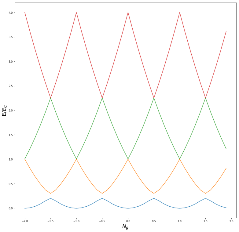
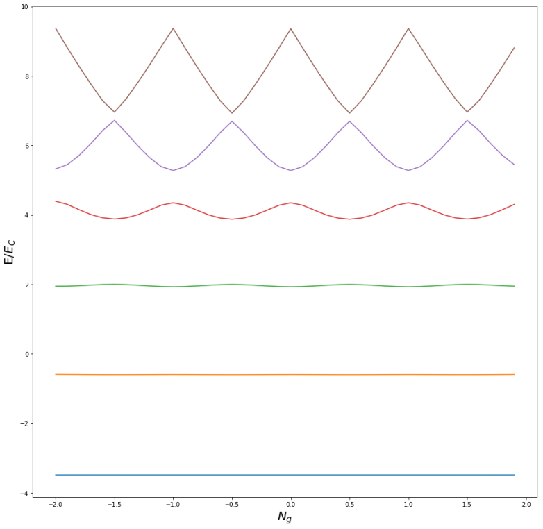
Learning Go with Kubernetes II – navigating structs, methods and interfaces

In the last post, we have set up our Go development environment and downloaded the Kubernetes Go client package. In this post, we will start to work on our first Go program which will retrieve and display a list of all nodes in a cluster.

You can download the full program here from my GitHub account. Copy this file to a subdirectory of the src directory in your Go workspace. You can build the program with

go build

which will create an executable called example1. If you run this (and have a working kubectl configuration pointing to a cluster with some nodes), you should see an output similar to the following.

$ ./example1 
NAME                  ARCH       OS
my-pool-7t62          amd64      Debian GNU/Linux 9 (stretch)
my-pool-7t6p          amd64      Debian GNU/Linux 9 (stretch)

Let us now go through the code step by step. In the first few lines, I declare my source code as part of the package main (which Go will search for the main entry point) and import a few packages that we will need later.

package main

import (
	"fmt"
	"path/filepath"
	metav1 "k8s.io/apimachinery/pkg/apis/meta/v1"
	"k8s.io/client-go/kubernetes"
	"k8s.io/client-go/tools/clientcmd"
	"k8s.io/client-go/util/homedir"
)

Note that the first two packages are Go standard packages, whereas the other four are Kubernetes packages. Also note that we import the package k8s.io/apimachinery/pkg/apis/meta/v1 using metav1 as an alias, so that an element foo in this package will be accessible as metav1.foo.

Next, we declare a function called main. As in many other program languages, the linker will use this function (in the package main) as an entry point for the executable.

func main() {
....
}

This function does not take any arguments and has no return values. Note that in Go, the return value is declared after the function name, not in front of the function name as in C or Java. Let us now take a look at the first three lines in the program

home := homedir.HomeDir()
kubeconfig := filepath.Join(home, ".kube", "config")
fmt.Printf("%-20s  %-10s %s\n", "NAME", "ARCH", "OS")

In the first line, we declare and initialize (using the := syntax) a variable called home. Variables in Go are strongly typed, but with this short variable declaration syntax, we ask the compiler to derive the type of the variable automatically from the assigned value.

Let us try to figure out this value. homedir is one of the packages that we have imported above. Using go list -json k8s.io/client-go/util/homedir, you can easily find the file in which this package is described. Let us look for a function HomeDir.

$ grep HomeDir $GOPATH/src/k8s.io/client-go/util/homedir/homedir.go 
// HomeDir returns the home directory for the current user
func HomeDir() string {

We see that there is a function HomeDir which returns a string, so our variable home will be a string. Note that the name of the function starts with an uppercase character so that it is exported by Go (in Go, elements starting with an uppercase character are exported, elements that start with a lowercase character not – you have to get used to this if you have worked with C or Java before). Applying the same exercise to the second line, you will find that kubeconfig is a string that is built from the three arguments to the function Join in the package filepath and path separators, i.e. this will be the path to the kubectl config file. Finally, the third line prints the header of the table of nodes we want to generate, in a printf-like syntax.

The next few lines in our code use the name of the kubectl config file to apply the configuration.

config, err := clientcmd.BuildConfigFromFlags("", kubeconfig)
if err != nil {
     panic(err)
}

This is again relatively straightforward, with one exception. The function BuildConfigFromFlags does actually return two values, as we can also see in its function declaration.

$ (cd  $GOPATH/src/k8s.io/client-go/tools/clientcmd ; grep "BuildConfigFromFlags" *.go)
client_config.go:// BuildConfigFromFlags is a helper function that builds configs from a master
client_config.go:func BuildConfigFromFlags(masterUrl, kubeconfigPath string) (*restclient.Config, error) {
client_config_test.go:	config, err := BuildConfigFromFlags("", tmpfile.Name())

The first argument is the actual configuration, the second is an error. We store both return values and check the error value – if everything went well, this should be nil which is the null value in Go.

Structures and methods

As a next step, we create a reference to the API client that we will use – a clientset.

clientset, err := kubernetes.NewForConfig(config)
if err != nil {
	panic(err)
}

Again, we can easily locate the function that we actually call here and try to determine its return type. By now, you should know how to figure out the directory in which we have to search for the answer.

$ (cd $GOPATH/src/k8s.io/client-go/kubernetes ; grep "func NewForConfig(" *.go)
clientset.go:func NewForConfig(c *rest.Config) (*Clientset, error) {

Now this is interesting for a couple of reasons. First, the first return value is of type *Clientset. This, like in C, is a pointer (yes, there are pointers in Go, but there is no pointer arithmetic), refering to the area in memory where an object is stored. The type of this object Clientset is not an elementary type, but seems to be a custom data type. If you search the file clientset.go in which the function is defined for the string Clientset, you will easy locate its definition.

// Clientset contains the clients for groups. Each group has exactly one
// version included in a Clientset.
type Clientset struct {
	*discovery.DiscoveryClient
	admissionregistrationV1beta1 *admissionregistrationv1beta1.AdmissionregistrationV1beta1Client
	appsV1                       *appsv1.AppsV1Client
	appsV1beta1                  *appsv1beta1.AppsV1beta1Client
...
	coreV1                       *corev1.CoreV1Client
...
}

where I have removed some lines for better readibility. So this is a structure. Similar to C, a structure is a sequence of named elements (field) which are bundled into one data structure. In the third line, for instance, we declare a field called appsV1 which is a pointer to an object of type appsv1.AppsV1Client (note that appsv1 is a package imported at the start of the file). The first line is a bit different – there is a field type, but not field name. This is called an embedded field, and its name is derived from the type name as the unqualified part of this name (in this case, this would be DiscoveryClient).

The field that we need from this structure is the field coreV1. However, there is a problem. Recall that only fields whose names start with an uppercase character are exported. So from outside the package, we cannot simply access this field using something like

clientset.coreV1

Instead, we need a function that returns this value which is located inside the package, something like a getter function. If you inspect the file clientset.go, you will easily locate the following function

// CoreV1 retrieves the CoreV1Client
func (c *Clientset) CoreV1() corev1.CoreV1Interface {
	return c.coreV1
}

This seems to be doing what we need, but its declaration is a bit unusual. There is a function name (CoreV1()), a return type (corev1.CoreV1Interface) and an empty parameter list. But there is also a declaration preceding the function name ((c *Clientset)).

This is called a receiver argument in Go. This binds our function to the type Clientset and at the same time acts as a parameter. When you invoke this function, you do it in the context of an instance of the type Clientset. In our example, we invoke this function as follows.

coreClient := clientset.CoreV1()

Here we call the function CoreV1 that we have just seen in clientset.go, passing a pointer to our instance clientset as the argument c. The function will then get the field coreV1 from this instance (which it can do, as it is located in the same package), and returns its value. Such a function could also accept additional parameters which are passed as usual. Note that the type of the receiver argument and the function need to be defined in the same package, otherwise the compiler would not know in which package it should look for the function CoreV1(). The presence of a receiver field turns a function into a method.

This looks a bit complicated, but is in fact rather intuitive (and those of you who have seen object oriented Perl know the drill). This construction links the structure Clientset containing data and the function CoreV1() with each other, under the umbrella of the package in which data type and function are defined. This comes close to a class in object-oriented programming languages.

Interfaces and inheritance

At this point, we hold the variable coreClient in our hands, and we know that it contains a (pointer to) an instance of the type k8s.io/client-go/kubernetes/typed/core/v1/CoreV1Interface. Resolving packages as before, we can now locate the file in which this type is declared.

$ (cd $GOPATH/src/k8s.io/client-go/kubernetes/typed/core/v1 ; grep "type CoreV1Interface" *.go)
core_client.go:type CoreV1Interface interface {

Hmm..this does not look like a structure. In fact, this is an interface. An interface defines a collection of methods (not just ordinary functions!). The value of an interface can be an instance of any type which implements all these methods, i.e. a type to which methods with the same names and signatures as those contained in the interface are linked using receiver arguments.

This sounds complicated, so let us look at a simple example from the corresponding section of “Tour in Go”.

type I interface {
	M()
}

type T struct {
	S string
}

// This method means type T implements the interface I,
// but we don't need to explicitly declare that it does so.
func (t T) M() {
	fmt.Println(t.S)
}

Here T is a structure containing a field S. The function M() has a receiver argument of type T and is therefore a method linked to the structure T. The interface I can be “anything on which we can call a method M“. Hence any variable to type T would be an admissible value for a variable of type I. In this sense, T implements I. Note that the “implements” relation is purely implicit, there is no declaration of implementation like in Java.

Let us now try to understand what this means in our case. If you locate the definition of the interface CoreV1Interface in core_client.go, you will see something like

type CoreV1Interface interface {
	RESTClient() rest.Interface
	ComponentStatusesGetter
	ConfigMapsGetter
...
	NodesGetter
...
}

The first line looks as expected – the interface contains a method RESTClient() returning a k8s.io/client-go/rest/Interface. However, the following lines do not look like method definitions. In fact, if you search the source code for these names, you will find that these are again interfaces! ConfigMapsGetter, for instance, is an interface declared in configmap.go which belongs to the same package and is defined as follows.

// ConfigMapsGetter has a method to return a ConfigMapInterface.
// A group's client should implement this interface.
type ConfigMapsGetter interface {
	ConfigMaps(namespace string) ConfigMapInterface
}

So this is a “real” interface. Its occurence in CoreV1Interface is an example of an embedded interface. This simply means that the interface CoreV1Interface contains all methods declared in ConfigMapsGetter plus all the other methods declared directly. This relation corresponds to interface inheritance in Java.

Among other interfaces, we find that CoreV1Interface embeds (think: inherits) the interface NodesGetter. Surprisingly, this is defined in node.go.

type NodesGetter interface {
	Nodes() NodeInterface
}

So we find that our variable coreClient contains something that – among other interfaces – implements the NodeGetter interface and therefore has a method called Nodes(). Thus we could do something like

coreClient.Nodes()

which would return an instance of the interface type NodeInterface. This in turn is declared in the same file, and we find that it has a method List()

type NodeInterface interface {
	Create(*v1.Node) (*v1.Node, error)
...	List(opts metav1.ListOptions) (*v1.NodeList, error)
...
}

This will return two things – an instance of NodeList and an error. NodeList is part of the package k8s.io/api/core/v1 and declared in types.go. To get this node list, we therefore need the following code.

nodeList, err := coreClient.Nodes().List(metav1.ListOptions{})

Note the argument to List – this is an anonymous instance of the type ListOptions which is just a structure, here we create an instance of this structure with all fields being nil and pass that instance as a parameter.

This completes our post for today. We have learned to navigate through structures, interfaces, methods and inheritance and how to locate type definitions and method signatures in the source code. In the next post, we will learn how to work with the node list, i.e. how to walk the list and prints its contents.

Learning Go with Kubernetes I – basics

When you work with Kubernetes and want to learn more about its internal workings and how to use the API, you will sooner or later reach the point at which the documentation can no longer answer all your questions and you need to consult the one and only source of truth – the source code of Kubernetes and a plethora of examples. Of course all of this is not written in my beloved Python (nor in C or Java) but in Go. So I decided to come up with a short series of posts that documents my own efforts to learn Go, using the Kubernetes source code as an example.

Note that this is not a stand-alone introduction into Go – there are many other sites doing this, like the Tour of Go on the official Golang home page, the free Golang book or many many blogs like Yourbasic. Rather, it is meant as an illustration of Go concepts for programmers with a background in a language like C (preferred), Java or Python which will help you to read and understand the Kubernetes server and client code.

What is Go(lang)?

Go – sometimes called Golang – is a programming language that was developed by Google engineers in an effort to create an easy to learn programming language well suited for programming fast, multithreaded servers and web applications. Some of its syntax and ideas actually remind me of C – there are pointers and structs – other of things I have seen in Python like slices. If you know any of these languages, you will find your way through the Go syntax quickly.

Go compiles code into native statically linked executables, which makes them easy to deploy. And Go comes with built-in support for multithreading, which makes it comparatively easy to build server-like applications. This blog lists some of the features of the Go language and compares them to concepts known from other languages.

Installation

The first thing, of course, is to install the Go environment. As Go is evolving rapidly, the packages offered by your distribution will most likely be outdated. To install the (fairly recent) version 1.10 on my Linux system, I have therefore downloaded the binary distribution using

wget https://dl.google.com/go/go1.10.8.linux-amd64.tar.gz
gzip -d go1.10.8.linux-amd64.tar.gz
tar xvf go1.10.8.linux-amd64.tar

in the directory where I wanted Go to be installed (I have used a subdirectory $HOME/Local for that purpose, but you might want to use /usr/local for a system-wide installation).

To resolve dependencies at compile time, Go uses a couple of standard directories – more on this below. These directories are stored in environment variables. To set these variables, add the following to your shell configuration script (.bashrc or .profile, depending on your system). Here GOROOT needs to point to the sub-directory go which the commands above will generate.

export GOROOT=directory-in-which-you-did-install-go/go
export GOPATH=$HOME/go
export PATH=$GOPATH/bin:$GOROOT/bin:$PATH

The most important executable in $GOROOT/bin is the go utility itself. This program can operate in various modes – go build will build a program, go get will install a package and so forth. You can run go help for a full list of available commands.

Packages and imports

A Go program is built from a collection of packages. Each source code file is part of a package, defined via the package declaration at the start of the file. Packages can be imported by other packages, which is the basis for reusable libraries. To resolve package names, Go has two different mechanisms – the GOPATH mode and the newer module mode available since Go 1.11. Here we will only discuss and use the old GOPATH mode.

In this mode, the essential idea is that your entire Go code is organized in a workspace, i.e. in one top-level directory, typically located in your home directory. In my case, my workspace is $HOME/go. To tell the Go build system about your workspace, you have to export the GOPATH environment variable.

export GOPATH=$HOME/go

The workspace directory follows a standard layout and typically contains the following subdirectories.

  • src – this is where all the source files live
  • pkg – here compiled versions of packages will be installed
  • bin – this is were executables resulting out of a build process will be moved

Let us try this out. Run the following commands to download the Kubernetes Go client package and some standard libraries.

go get k8s.io/client-go/...
go get golang.org/x/tools/...

When this has completed, let us take a look at our GOPATH directory to see what has happened.

$ ls $GOPATH/src
github.com  golang.org  gopkg.in  k8s.io

So the Go utility has actually put the source code of the downloaded package into our workspace. As GOPATH points to this workspace, the Go build process can resolve package names and map them into this workspace. If, for instance, we refer to the package k8s.io/client-go/kubernetes in our source code (as we will do it in the example later on), the Go compiler will look for this package in

GOPATH/src/k8s.io/client-go/kubernetes

To get information on a package, we can use the list command of the Go utility. Let us try this out.

$ go list -json k8s.io/client-go/kubernetes
{
	"Dir": "[REDACTED - this is $GOPATH]/src/k8s.io/client-go/kubernetes",
	"ImportPath": "k8s.io/client-go/kubernetes",
	"ImportComment": "k8s.io/client-go/kubernetes",
        [REDACTED - SOME MORE LINES]
	"Root": "[REDACTED - THIS SHOULD BE $GOROOT]",
	"GoFiles": [
		"clientset.go",
		"doc.go",
		"import.go"
	],
[... REDACTED - MORE OUTPUT ...]

Here I have removed a few lines and redacted the output a bit. We see that the Dir field is the directory in which the compiler will look for the code constituting the package. The top-level directory is the directory to which GOPATH points. The import path is the path that an import statement in a program using this package would be. The list GoFiles is a list of all files that are parts of this package. If you inspect these files, you will in fact find that the first statement they contain is

package kubernetes

indicating that they belong to the Kubernetes package. You will see that the package name (defined in the source code) equals the last part of the full import path (part of the filesystem structure) by convention (which, as far as I understand, is not enforced technically).

I recommend to spend some time reading more on typical layouts of Go packages here ore here.

We have reached the end of our first post in this series. In the next post, we will write our first example program which will list nodes in a Kubernetes cluster.

Kubernetes on your PC: playing with minikube

In my previous posts on Kubernetes, I have used public cloud providers like AWS or DigitalOcean to spin up test clusters. This is nice and quite flexible – you can create clusters with an arbitrary numbers of nodes, can attach volumes, create load balancers and define networks. However, cloud providers will of course charge for that, and your freedom to adapt the configuration and play with the management nodes is limited. It would be nice to have a playground, maybe even on your own machine, which gives you a small environment to play with. This is exactly what the minikube project is about.

Basics and installation

Minikube is a set of tools that allows you to easily create a one-node Kubernetes cluster inside a virtual machine running on your PC. Thus there is only one node, which serves at the same time as a management node and a worker node. Minikube supports several virtualization toolsets, but the default (both on Linux and an Windows) is Virtualbox. So as a first step, let us install this.

$ sudo apt-get install virtualbox

Next, we can install minikube. We will use release 1.0 which has been published end of march. Minikube is one single, statically linked binary. I keep third-party binaries in a directory ~/Local/bin, so I applied the following commands to download and install minikube.

$ curl -Lo minikube https://storage.googleapis.com/minikube/releases/v1.0.0/minikube-linux-amd64 
$ chmod 700 minikube
$ mv minikube ~/Local/bin

Running minikube

Running minikube is easy – just execute

$ minikube start

When you do this for the first time after installation, Minikube needs to download a couple of images. These images are cached in ~/minikube/cache and require a bit more than 2 Gb of disk space, so this will take some time.

Once the download is complete, minikube will bring up a virtual machine, install Kubernetes in it and adapt your kubectl configuration to point to this newly created cluster.

By default, minikube will create a virtual machine with two virtual CPUs (i.e. two hyperthreads) and 2 GB of RAM. This is the minimum for a reasonable setup. If you have a machine with sufficient memory, you can allocate more. To create a machine with 4 GB RAM and four CPUs, use

$ minikube start --memory 4096 --cpus 4

Let us see what this command does. If you print your kubectl config file using kubectl config view, you will see that minikube has added a new context to your configuration and set this context as the default context, while preserving any previous configuration that you had. Next, let us inspect our nodes.

$ kubectl get nodes
NAME       STATUS   ROLES    AGE     VERSION
minikube   Ready    master   3m24s   v1.14.0

We see that there is one node, as expected. This node is a virtual machine – if you run virtualbox, you will be able to see that machine and its configuration.

screenshot-from-2019-04-08-14-06-02.png

When you run minikube stop, the virtual machine will be shut down, but will survive. When you restart minikube, this machine will again be used.

There are several ways to actually log into this machine. First, minikube has a command that will do that – minikube ssh. This will log you in as user docker, and you can do a sudo -s to become root.

Alternatively, you can stop minikube, then start the machine manually from the virtualbox management console, log into it (user “docker”, password “tcuser” – it took me some time to figure this out, if you want to verify this look at this file, read the minikube Makefile to confirm that the build uses buildroot and take a look at the description in this file) and then start minikube. In this case, minikube will detect that the machine is already running.

Networking in Minikube

Let us now inspect the networking configuration of the virtualbox instance that minikube has started for us. When minikube comes up, it will print a message like the following

“minikube” IP address is 192.168.99.100

In case you missed this message, you can use run minikube ip to obtain this IP address. How is that IP address reachable from the host?

If you run ifconfig and ip route on the host system, you will find that virtualbox has created an additional virtual network device vboxnet0 (use ls -l /sys/class/net to verify that this is a virtual device) and has added a route sending all the traffic to the CIDR range 192.168.99.0/24 to this device, using the source IP address 192.168.99.1 (the src field in the output of ip route). So this gives you yet another way to SSH into the virtual machine

ssh docker@$(minikube ip)

showing also that the connection works.

Inside the VM, however, the picture is a bit more complicated. As a starting point, let us print some details on the virtual machine that minikube has created.

$ vboxmanage showvminfo  minikube --details | grep "NIC" | grep -v "disabled"
NIC 1:           MAC: 080027AE1062, Attachment: NAT, Cable connected: on, Trace: off (file: none), Type: virtio, Reported speed: 0 Mbps, Boot priority: 0, Promisc Policy: deny, Bandwidth group: none
NIC 1 Settings:  MTU: 0, Socket (send: 64, receive: 64), TCP Window (send:64, receive: 64)
NIC 1 Rule(0):   name = ssh, protocol = tcp, host ip = 127.0.0.1, host port = 44359, guest ip = , guest port = 22
NIC 2:           MAC: 080027BDDBEC, Attachment: Host-only Interface 'vboxnet0', Cable connected: on, Trace: off (file: none), Type: virtio, Reported speed: 0 Mbps, Boot priority: 0, Promisc Policy: deny, Bandwidth group: none

So we find that virtualbox has equipped our machine with two virtual network interfaces, called NIC 1 and NIC 2. If you ssh into the machine, run ifconfig and compare the MAC address values, you fill find that these two devices appear as eth0 and eth1.

Let us first take a closer look at the first interface. This is a so-called NAT device. Basically, this device acts like a router – when a TCP/IP packet is sent to this device, the virtualbox engine extracts the data, opens a port on the host machine and sends the data to the target host. When the answer is received, another address translation is performed and the packet is fed again into the virtual device.

Much like an actual router, this mechanism makes it impossible to reach the virtual machine from the host – unless a port forwarding rule is set up. If you look at the output above, you will see that there is one port forwarding rule already in place, mapping the SSH port of the guest system to a port on the host, in our case 44359. When you run netstat on the host, you will find that minikube itself actually connects to this port to reach the SSH daemon inside the virtual machine – and, incidentally, this gives us yet another way to SSH into our machine.

ssh -p 44359 docker@127.0.0.1

Now let us turn to the second interface – eth1. This is an interface type which the VirtualBox documentation refers to as host-only networking. In this mode, an additional virtual network device is created on the host system – this is the vboxnet0 device which we have already spotted. Traffic sent to the virtual device eth1 in the machine is forwarded to this device and vice versa (this is in fact handled by a special driver vboxnet as you can tell from the output of ethtool -i vboxnet0). In addition, VirtualBox has added routes on the host and the guest system to connect this device to the network 192.168.99.0/24. Note that this network is completely separated from the host network. So our picture looks as follows.

VirtualBoxNetworking

What does this mean for Kubernetes networking in Minikube? Well, the first obvious consequence is that we can use node ports to access services from our host system. Let us try this out, using the examples from a previous post.

$ kubectl apply -f https://raw.githubusercontent.com/christianb93/Kubernetes/master/pods/deployment.yaml
deployment.apps/alpine created
$ kubectl apply -f https://raw.githubusercontent.com/christianb93/Kubernetes/master/network/nodePortService.yaml
service/alpine-service created
$ kubectl get svc
NAME             TYPE        CLUSTER-IP      EXTERNAL-IP   PORT(S)          AGE
alpine-service   NodePort    10.99.112.157           8080:32197/TCP   26s
kubernetes       ClusterIP   10.96.0.1               443/TCP          4d17h

So our service has been created and is listening on the node port 32197. Let us see whether we can reach our service from the host. On the host, open a terminal window and enter

$ nodeIP=$(minikube ip)
$ curl $nodeIP:32197
<h1>It works!</h1>

So node port services work as expected. What about load balancer services? In a typical cloud environment, Kubernetes will create load balancers whenever we set up a load balancer service that is reachable from outside the cluster. Let us see what the corresponding behavior in a minikube environment is.

$ kubectl delete svc alpine-service
service "alpine-service" deleted
$ kubectl apply -f https://raw.githubusercontent.com/christianb93/Kubernetes/master/network/loadBalancerService.yaml
service/alpine-service created
$ kubectl get svc
NAME             TYPE           CLUSTER-IP       EXTERNAL-IP   PORT(S)          AGE
alpine-service   LoadBalancer   10.106.216.127        8080:31282/TCP   3s
kubernetes       ClusterIP      10.96.0.1                443/TCP          4d18h
$ curl $nodeIP:31282
<h1>It works!</h1>

You will find that even after a few minutes, the external IP remains pending. Of course, we can still reach our service via the node port, but this is not the idea of a load balancer service. This is not awfully surprising, as there is no load balancer infrastructure on your local machine.

However, minikube does offer a tool that allows you to emulate a load balancer – minikube tunnel. To see this in action, open a second terminal on your host and enter

minikube tunnel

After a few seconds, you will be asked for your root password, as minikube tunnel requires root privileges. After providing this, you should see some status message on the screen. In our first terminal, we can now inspect our service again.

$ kubectl get svc alpine-service
NAME             TYPE           CLUSTER-IP       EXTERNAL-IP      PORT(S)          AGE
alpine-service   LoadBalancer   10.106.216.127   10.106.216.127   8080:31282/TCP   17m
$ curl 10.106.216.127:8080
<h1>It works!</h1>

Suddenly, the field external IP is populated, and we can reach our service under this IP address and the port number that we have configured in our service description. What is going on here?

To find the answer, we can use ip route on the host. If you run this, you will find that minikube has added an additional route which looks as follows.

10.96.0.0/12 via 192.168.99.100 dev vboxnet0 

Let us compare this with the CIDR range that minikube uses for services.

$ kubectl cluster-info dump | grep -m 1 range
                            "--service-cluster-ip-range=10.96.0.0/12",

So minikube has added a route that will forward all traffic directed towards the IP ranged used for Kubernetes services to the IP address of the VM in which minikube is running, using the virtual ethernet device created for this VM. Effectively, this sets up the VM as a gateway which makes it possible to reach this CIDR range (see also the minikube documentation for details). In addition, minikube will set the external IP of the service to the cluster IP address, so that the service can now be reached from the host (you can also verify the setup using ip route get 10.106.216.127 to display the result of the route resolution process for this destination).

Note that if you stop the separate tunnel process again, the additional route disappears again and the external IP address of the service switches back to “pending”.

Persistent storage in Minikube

We have seen in my previous posts on persistent storage that cloud platforms typically define a default storage class and offer a way to automatically create persistent volumes for a PVC. The same is true for minikube – there is a default storage class.

$ kubectl get storageclass
NAME                 PROVISIONER                AGE
standard (default)   k8s.io/minikube-hostpath   5d1h

In fact, minikube is by default starting a custom storage controller (as you can check by running kubectl get pods -n kube-system). To understand how this storage controller is operating, let us construct a PVC and analyse the resulting volume.

$ kubectl apply -f - << EOF
apiVersion: v1
kind: PersistentVolumeClaim
metadata:
  name: my-pvc
  namespace: default
spec:
  accessModes:
    - ReadWriteOnce
  resources:
    requests:
      storage: 512Mi
EOF

If you use kubectl get pv, you will see that the storage controller has created a new persistent volume. Let us attach this volume to a container to play with it.

$ kubectl apply -f - << EOF
apiVersion: v1
kind: Pod
metadata:
  name: pv-test
  namespace: default
spec:
  containers:
  - name: pv-test-ctr
    image: httpd:alpine
    volumeMounts:
      - mountPath: /test
        name: test-volume
  volumes:
  - name: test-volume
    persistentVolumeClaim:
      claimName: my-pvc
EOF

If you then use once more SSH into the VM, you should see our new container running. Using docker inspect, you will find that Docker has again created a bind mount, binding the mount point /test to a directory on the host named /tmp/hostpath-provisioner/pvc-*, where * indicates some randomly generated number. When you attach to the container and create a file /test/myfile, and then display the contents of this directory in the VM, you will in fact see that the file has been created.

So at the end of the day, a persistent volume in minikube is simply a host-path volume, pointing to a directory on the one and only node used by minikube. Also note that this storage is really persistent in the sense that it survives a restart of minikube.

Additional features

There are a view additional features of minikube that are worth being mentioned. First, it is very easy to install an NGINX ingress controller – the command

minikube addons enable ingress

will do this for you. Second, minikube also allows you to install and enable the Kubernetes dashboard. In fact, running

minikube dashboard

will install the dashboard and open a browser pointing to it.

KubernetesDashboard

And there are many more addons- you can get a full list with minikube addons list or in the minikube documentation. I highly recommend to browse that list and play with one of them.

Automating cluster creation on DigitalOcean

So far I have mostly used Amazons EKS platform for my posts on Kubernetes. However, this is of course not the only choice – there are many other providers that offer Kubernetes in a cloud environment. One of them which is explicitly targeting developers is DigitalOcean. In this post, I will show you how easy it is to automate the creation of a Kubernetes cluster on the DigitalOcean platform.

Creating an SSH key

Similar to most other platforms, DigitalOcean offers SSH access to their virtual machines. You can either ask DigitalOcean to create a root password for you and send it to you via mail, or – preferred – you can use SSH keys.

Different from AWS, key pairs need to be generated manually outside of the platform and imported. So let us generate a key pair called do_k8s and import it into the platform. To create the key locally, run

$ ssh-keygen -f ~/.ssh/do_k8s -N ""

This will create a new key (not protected by a passphrase, so be careful) and store the private key file and the public key file in separate files in the SSH standard directory. You can print out the contents of the public key file as follows.

$ cat ~/.ssh/do_k8s.pub

The resulting output is the public part of your SSH key, including the string “ssh-rsa” at the beginning. To make this key known to DigitalOcean, log into the console, navigate to the security tab, click “Add SSH key”, enter the name “do_k8s” and copy the public key into the corresponding field.

Next, let us test our setup. We will create a request using curl to list all our droplets. In the DigitalOcean terminology, a droplet is a virtual machine instance. Of course, we have not yet created one, so expect to get an empty list, but we can uses this to test that our token works. For that purpose, we simply use curl to direct a GET request to the API endpoint and pass the bearer token in an additional header.

$ curl -s -X\
     GET "https://api.digitalocean.com/v2/droplets/"\
     -H "Authorization: Bearer $bearerToken"\
     -H "Content-Type: application/json"
{"droplets":[],"links":{},"meta":{"total":0}}

So no droplets, as expected, but our token seems to work.

Droplets

Let us now see how we can create a droplet. We could of course also use the cloud console to do this, but as our aim is automation, we will leverage the API.

When you have worked with a REST API before, you will not be surprised to learn that this is done by submitting a POST request. This request will contain a JSON body that describes the resource to be created – a droplet in our case – and a header that, among other things, is used to submit the bearer token that we have just created.

To be able to log into our droplet later on, we will have to pass the SSH key that we have just created to the API. Unfortunately, for that, we cannot use the name of the key (do_k8s), but we will have to use the internal ID. So the first thing we need to do is to place a GET request to extract this ID. As so often, we can do this with a combination of curl to retrieve the key and jq to parse the JSON output.

$ sshKeyName="do_k8s"
$ sshKeyId=$(curl -s -X \
      GET "https://api.digitalocean.com/v2/account/keys/" \
      -H "Authorization: Bearer $bearerToken" \
      -H "Content-Type: application/json" \
       | jq -r "select(.ssh_keys[].name=\"$sshKeyName\") .ssh_keys[0].id")

Here we first use curl to get a list of all keys in JSON format. We then pipe the output into jq and use the select statement to get only those items for which the attribute name matches our key name. Finally, we extract the ID field from this item and store it in a shell variable.

We can now assemble the data part of our request. The code is a bit difficult to read, as we need to escape quotes.

$ data="{\"name\":\"myDroplet\",\
       \"region\":\"fra1\",\
       \"size\":\"s-1vcpu-1gb\",\
       \"image\":\"ubuntu-18-04-x64\",\
       \"ssh_keys\":[ $sshKeyId ]}"

To get a nice, readable representation of this, we can use jq’s pretty printing capabilities.

$ echo $data | jq
{
  "name": "myDroplet",
  "region": "fra1",
  "size": "s-1vcpu-1gb",
  "image": "ubuntu-18-04-x64",
  "ssh_keys": [
    24322857
  ]
}

We see that this is a simple JSON structure. There is a name, which will be the name used later in the DigitalOcean console to display our droplet, a region (I use fra1 in central europe, a full list of all available regions is here), a size specifying the type of the droplet (in this case one vCPU and 1 GB), the OS image to use and finally the SSH key id that we have extracted before. Let us now submit our creation request.

$ curl -s  -X \
      POST "https://api.digitalocean.com/v2/droplets"\
      -d "$data" \
      -H "Authorization: Bearer $bearerToken"\
      -H "Content-Type: application/json"

When everything works, you should see your droplet on the DigitalOcean web console. If you repeat the GET request above to obtain all droplets, your droplet should also show up in the list. To format the output, you can again pipe it through jq. After some time, the status field (located at the top of the output) should be “active”, and you should be able to retrieve an IP address from the section “networks”. In my case, this is 46.101.128.54. We can now SSH into the machine as follows.

$ ssh -i ~/.ssh/do_key root@46.101.128.54

Needless to say that it is also easy to delete a droplet again using the API. A full reference can be found here. I have also created a few scripts that can automatically create a droplet, list all running droplets and delete a droplet.

Creating a Kubernetes cluster

Let us now turn to the creation of a Kubernetes cluster. The good news is that this is even easier than the creation of a droplet – a single POST request will do!

But before we can assemble our request, we need to understand how the cluster definition is structured. Of course, a Kubernetes cluster consists of a couple of management nodes (which DigitalOcean manages for you in the background) and worker nodes. On DigitalOcean, worker nodes are organized in node pools. Each node pool contains a set of identical worker nodes. We could, for instance, create one pool with memory-heavy machines for database workloads that require caching, and a second pool with general purpose machines for microservices. The smallest machines that DigitalOcean will allow you to bring up as worker nodes are of type s-1vcpu-2gb. To fully specify a node pool with two machines of this type, the following JSON fragment is used.

$ nodePool="{\"size\":\"s-1vcpu-2gb\",\
      \"count\": 2,\
      \"name\": \"my-pool\"}"
$ echo $nodePool | jq
{
  "size": "s-1vcpu-2gb",
  "count": 2,
  "name": "my-pool"
}

Next, we assemble the data part of the POST request. We will need to specify an array of node pools (here we will use only one node pool), the region, a name for the cluster, and a Kubernetes version (you can of course ask the API to give you a list of all existings versions by running a GET request on the URL path/v2/kubernetes/options). Using the node pool snippet from above, we can assemble and display our request data as follows.

$ data="{\"name\": \"my-cluster\",\
        \"region\": \"fra1\",\
        \"version\": \"1.13.5-do.1\",\
        \"node_pools\": [ $nodePool ]}"
$ echo $data | jq
{
  "name": "my-cluster",
  "region": "fra1",
  "version": "1.13.5-do.1",
  "node_pools": [
    {
      "size": "s-1vcpu-2gb",
      "count": 2,
      "name": "my-pool"
    }
  ]
}

Finally, we submit this data using a POST request as we have done it for our droplet above.

$ curl -s -w -X\
    POST "https://api.digitalocean.com/v2/kubernetes/clusters"\
    -d "$data" \
    -H "Authorization: Bearer $bearerToken"\
    -H "Content-Type: application/json"

Now cluster creation should start, and if you navigate to the Kubernetes tab of the DigitalOcean console, you should see your cluster being created.

Cluster creation is rather fast on DigitalOcean, and typically takes less than five minutes. To complete the setup, you will have to download the kubectl config file for the newly generated cluster. Of course, there are again two ways to do this – you can use the web console or the API. I have created a script that fully automates cluster creation – it detects the latest Kubernetes version, creates the cluster, waits until it is active and downloads the kubectl config file for you. If you run this, make sure to populate the shell variable bearerToken with your token or use the -t switch to pass the token to the script. The same directory also contains a few more scripts to list all existing clusters and to delete them again.

Stateful sets with Kubernetes

In one of my previous posts, we have looked at deployment controllers which make sure that a certain number of instances of a given pod is running at all times. Failures of pods and nodes are automatically detected and the pod is restarted. This mechanism, however, only works well if the pods are actually interchangeable and stateless. For stateful pods, additional mechanisms are needed which we discuss in this post.

Simple stateful sets

As a reminder, let us first recall some properties of deployments aka stateless sets in Kubernetes. For that purpose, let us create a deployment that brings up three instances of the Apache httpd.

$ kubectl apply -f - << EOF
apiVersion: apps/v1
kind: Deployment
metadata:
  name: httpd
spec:
  selector:
    matchLabels:
      app: httpd
  replicas: 3
  template:
    metadata:
      labels:
        app: httpd
    spec:
      containers:
        - name: httpd-ctr
          image: httpd:alpine
EOF
deployment.apps/httpd created
$ $ kubectl get pods
NAME                     READY   STATUS    RESTARTS   AGE
httpd-76ff88c864-nrs8q   1/1     Running   0          12s
httpd-76ff88c864-rrxw8   1/1     Running   0          12s
httpd-76ff88c864-z9fjq   1/1     Running   0          12s

We see that – as expected – Kubernetes has created three pods and assigned random names to them, composed of the name of the deployment and a random string. We can run hostname inside one of the containers to verify that these are also the hostnames of the pods. Let us pick the first pod.

$ kubectl exec -it httpd-76ff88c864-nrs8q hostname
httpd-76ff88c864-nrs8q

Let us now kill the first pod.

$ kubectl delete pod httpd-76ff88c864-nrs8q

After a few seconds, a new pod is created. Note, however, that this pod receives a new pod name and also a new host name. And, of course, the new pod will receive a new IP address. So its entire identity – hostname, IP address etc. – has changed. Kubernetes did not actually magically revive the pod, but it realized that one pod was missing in the set and simply created a new pod according to the same pod specification template.

This behavior allows us to recover from a simple pod failure very quickly. It does, however, pose a problem if you want to deploy a set of pods that each take a certain role and rely on stable identities. Suppose, for instance, that you have an application that comes in pairs. Each instance needs to connect to a second instance, and to do this, it needs to know the name of that instance name and needs to rely on the stability of that name. How would you handle this with Kubernetes?

Of course, we could simply define two pods (not deployments) and use different names for both deployments. In addition, we could set up a service for each pod, which will create DNS entries in the Kubernetes internal DNS network. This would allow each pod to locate the second pod in the pair. But of course this is cumbersome and requires some additional monitoring to detect failures and restart pods. Fortunately, Kubernetes did introduce an alternative known as Stateful sets.

In some sense, a stateful set is similar to a deployment. You define a pod template and a desired number of replicas. A controller will then bring up these replicas, monitor them and replace them in case of a failure. The difference between a stateful set and a deployment is that each instance in a stateful set receives a unique identity which is stable across restarts. In addition, the instances of a stateful set are brought up and terminated in a defined order.

This is best explained using an example. So let us define a stateful set that contains three instances of a HTTPD (which, of course, is a toy example and not a typical application for which you would use stateful sets).

$ kubectl apply -f - << EOF
apiVersion: v1
kind: Service
metadata:
  name: httpd-svc
spec:
  clusterIP: None
  selector:
    app: httpd
---
apiVersion: apps/v1
kind: StatefulSet
metadata:
  name: stateful-test
spec:
  selector:
    matchLabels:
      app: httpd
  replicas: 3 
  serviceName: httpd-svc
  template:
    metadata:
      labels:
        app: httpd
    spec:
      containers:
      - name: httpd-ctr
        image: httpd:alpine
EOF
service/httpd-svc created
statefulset.apps/stateful-test created

That is a long manifest file, so let us go through it one by one. The first part of the file is simply a service called httpd-svc. The only thing that might seem strange is that this service has no cluster IP. This type of service is called a headless service. Its primary purpose is not to serve as a load balancer for pods (which would not make sense anyway in a typical stateful scenario, as the pods are not interchangeable), but to provide a domain in the cluster internal DNS system. We will get back to this point in a few seconds.

The second part of the manifest file is the specification of the actual stateful set. The overall structure is very similar to a deployment – there is the usual metadata section, a selector that selects the pods belonging to the set, a replica count and a pod template. However, there is also a reference serviceName to the headless service that we have just created.

Let us now inspect our cluster to see that this manifest file has created. First, of course, there is the service that the first part of our manifest file describes.

$ kubectl get svc httpd-svc
NAME        TYPE        CLUSTER-IP   EXTERNAL-IP   PORT(S)   AGE
httpd-svc   ClusterIP   None                     13s

As expected, there is no cluster IP address for this service and no port. In addition, we have created a stateful set that we can inspect using kubectl.

$ $ kubectl get statefulset stateful-test
NAME            READY   AGE
stateful-test   3/3     88s

The output looks similar to a deployment – we see that our stateful set has three replicas out of three in total in status READY. Let us inspect those pods. We know that, by definition, our stateful set consists of all pods that have an app label with value equal to httpd, so we can use a label selector to list all these pods.

$ kubectl get pods -l app=httpd 
NAME              READY   STATUS    RESTARTS   AGE
stateful-test-0   1/1     Running   0          4m28s
stateful-test-1   1/1     Running   0          4m13s
stateful-test-2   1/1     Running   0          4m11s

So there are three pods that belong to our set, all in status running. However, note that the names of the pods follow a different pattern than for a deployment. The name is composed of the name of the stateful set plus an ordinal, starting at zero. Thus the names are predictable. In addition, the AGE field tells you that Kubernetes will also bring up the pods in this order, i.e. it will start pod stateful-test-0, wait until this pod is ready, then bring up the second pod and so on. If you delete the set again, it will bring them down in the reverse order.

StatefulSetI

Let us check whether the pod names are not only predictable, but also stable. To do this, let us bring down one pod.

$ kubectl delete pod stateful-test-1
pod "stateful-test-1" deleted
$ kubectl get pods -l app=httpd 
NAME              READY   STATUS              RESTARTS   AGE
stateful-test-0   1/1     Running             0          8m41s
stateful-test-1   0/1     ContainerCreating   0          2s
stateful-test-2   1/1     Running             0          8m24s

So Kubernetes will bring up a new pod with the same name again – our names are stable. The IP addresses, however, are not guaranteed to remain stable and typically change if a pod dies and a substitute is created. So how would the pods in the set communicate with each other, and how would another pod communicate with one of them?

To solve this, Kubernetes will add DNS records for each pod. Recall that as part of a Kubernetes cluster, a DNS server is running (with recent versions of Kubernetes, this is typically CoreDNS). Kubernetes will mount the DNS configuration file /etc/resolv.conf into each of the pods so that the pods use this DNS server. For each pod in a stateful set, Kubernetes will add a DNS record. Let us use the busybox image to show this record.

$ kubectl run -i --tty --image busybox:1.28 busybox --restart=Never --rm
If you don't see a command prompt, try pressing enter.
/ # cat /etc/resolv.conf
nameserver 10.245.0.10
search default.svc.cluster.local svc.cluster.local cluster.local
options ndots:5
/ # nslookup stateful-test-0.httpd-svc
Server:    10.245.0.10
Address 1: 10.245.0.10 kube-dns.kube-system.svc.cluster.local

Name:      stateful-test-0.httpd-svc
Address 1: 10.244.0.108 stateful-test-0.httpd-svc.default.svc.cluster.local

What happens? Apparently Kubernetes creates one DNS record for each pod in the stateful set. The name of that record is composed of the pod name, the service name, the namespace in which the service is defined (the default namespace in our case), the subdomain svc in which all entries for services are stored and the cluster domain. Kubernetes will also add a record for the service itself.

/ # nslookup httpd-svc
Server:    10.245.0.10
Address 1: 10.245.0.10 kube-dns.kube-system.svc.cluster.local

Name:      httpd-svc
Address 1: 10.244.0.108 stateful-test-0.httpd-svc.default.svc.cluster.local
Address 2: 10.244.0.17 stateful-test-1.httpd-svc.default.svc.cluster.local
Address 3: 10.244.1.49 stateful-test-2.httpd-svc.default.svc.cluster.local

So we find that Kubernetes has added additional A records for the service, corresponding to the three pods that are part of the stateful set. Thus an application could either look up one of the services directly, or use round-robin and a lookup of the service name to talk to the pods.

As a sidenote, you have really have to use version 1.28 of the busybox image to make this work – later versions seem to have a broken nslookup implementation, see this issue for details.

Stateful sets and storage

Stateful sets are meant to be used for applications that store a state, and of course they typically do this using persistent storage. When you create a stateful set with three replicas, you would of course want to attach storage to each of them, but of course you want to use different volumes. In case a pod is lost and restarted, you would also want to automatically attach the pod to the same volume to which the pod it replaces was attached. All this is done using PVC templates.

Essentially, a PVC template has the same role for storage that a pod specification template has for pods. When Kubernetes creates a stateful set, it will use this template to create a set of persistent volume claims, one for each member of the set. These persistent volume claims are then bound to volumes, either manually created volumes or dynamically provisioned volumes. Here is an extension of our previously used example that includes PVC templates.

apiVersion: v1
kind: Service
metadata:
  name: httpd-svc
spec:
  clusterIP: None
  selector:
    app: httpd
---
apiVersion: apps/v1
kind: StatefulSet
metadata:
  name: stateful-test
spec:
  selector:
    matchLabels:
      app: httpd
  replicas: 3 
  serviceName: httpd-svc
  template:
    metadata:
      labels:
        app: httpd
    spec:
      containers:
      - name: httpd-ctr
        image: httpd:alpine
        volumeMounts:
        - name: my-pvc
          mountPath: /test
  volumeClaimTemplates:
  - metadata:
      name: my-pvc
    spec:
      accessModes:
      - ReadWriteOnce
      resources:
        requests:
          storage: 1Gi

The code is the same as above, with two differences. First, we have an additional array called volumeClaimTemplates. If you consult the API reference, you will find that the elements of this array are of type PersistentVolumeClaim and therefore follow the same syntax rules as the PVCs discussed in my previous posts.

The second change is that in the container specification, there is a mount point. This mount point refers directly to the PVC name, not using a volume on Pod level as a level of indirection as for ordinary deployments.

When we apply this manifest file and display the existing PVCs, we will find that for each instance of the stateful set, Kubernetes has created a PVC.

$ kubectl get pvc
NAME                     STATUS   VOLUME                                     CAPACITY   ACCESS MODES   STORAGECLASS   AGE
my-pvc-stateful-test-0   Bound    pvc-78bde820-53e0-11e9-b859-0afa21a383ce   1Gi        RWO            gp2            1m
my-pvc-stateful-test-1   Bound    pvc-8790edc9-53e0-11e9-b859-0afa21a383ce   1Gi        RWO            gp2            38s
my-pvc-stateful-test-2   Bound    pvc-974cc9fa-53e0-11e9-b859-0afa21a383ce   1Gi        RWO            gp2            12s

StatefulSetII

We see that again, the naming of the PVCs follows a predictable patterns and is composed of the PVC template name and the name of the corresponding pod in the stateful set. Let us now look at one of the pods in greater detail.

$ kubectl describe pod stateful-test-0
Name:               stateful-test-0
Namespace:          default
Priority:           0
[ --- SOME LINES REMOVED --- ]
Containers:
  httpd-ctr:
[ --- SOME LINES REMOVED --- ]
    Mounts:
      /test from my-pvc (rw)
      /var/run/secrets/kubernetes.io/serviceaccount from default-token-kfwxf (ro)
[ --- SOME LINES REMOVED --- ]
Volumes:
  my-pvc:
    Type:       PersistentVolumeClaim (a reference to a PersistentVolumeClaim in the same namespace)
    ClaimName:  my-pvc-stateful-test-0
    ReadOnly:   false
  default-token-kfwxf:
    Type:        Secret (a volume populated by a Secret)
    SecretName:  default-token-kfwxf
    Optional:    false
[ --- SOME LINES REMOVED --- ]

Thus we find that Kubernetes has automatically created a volume called my-pvc (the name of the PVC template) in each pod. This pod volume then refers to the instance-specific PVC which again refers to the volume, and this pod volume is in turn referenced by the Docker mount point.

What happens if a pod goes down and is recreated? Let us test this by writing an instance specific file onto the volume mounted by pod #0, deleting the pod, waiting for a few seconds to give Kubernetes enough time to recreate the pod and checking the content of the volume.

$ kubectl exec -it stateful-test-0 touch /test/I_am_number_0
$ kubectl exec -it stateful-test-0 ls /test
I_am_number_0  lost+found
$ kubectl delete pod stateful-test-0 && sleep 30
pod "stateful-test-0" deleted
$ kubectl exec -it stateful-test-0 ls /test
I_am_number_0  lost+found

So we see that in fact, Kubernetes has bound the same volume to the replacement for pod #0 so that the application can access the same data again. The same happens if we forcefully remove the node – the volume is then automatically attached to the node on which the replacement pod will be scheduled. Note, however, that this only works if the new node is in the same availability zone as the previous node as on most cloud platforms, cross-AZ attachment of volumes to nodes is not possible, in this case, the scheduler will have to wait until a new node in that zone has been brought up (see e.g. this link for more information on running Kubernetes in multiple zones).

Let us continue to investigate the life cycle of our volumes. We have seen that the volumes have been created automatically when the stateful set was created. The converse, however, is not true.

$ kubectl delete statefulset stateful-test
statefulset.apps "stateful-test" deleted
$ kubectl delete svc httpd-svc
service "httpd-svc" deleted
$ kubectl get pvc
NAME                     STATUS   VOLUME                                     CAPACITY   ACCESS MODES   STORAGECLASS   AGE
my-pvc-stateful-test-0   Bound    pvc-78bde820-53e0-11e9-b859-0afa21a383ce   1Gi        RWO            gp2            14m
my-pvc-stateful-test-1   Bound    pvc-8790edc9-53e0-11e9-b859-0afa21a383ce   1Gi        RWO            gp2            13m
my-pvc-stateful-test-2   Bound    pvc-974cc9fa-53e0-11e9-b859-0afa21a383ce   1Gi        RWO            gp2            13m

So the persistent volume claims (and the volumes) remain existent if the delete the stateful set. This seems to be a deliberate design decision to give the administrator a chance to copy or backup the data on the volumes even after the set has been deleted. To fully clean up the volumes, we therefore need to delete the PVCs manually. Fortunately, this can again be done using a label selector, in our case

kubectl delete pvc -l app=httpd

will do the trick. Note that it is even possible to reuse the PVCs – in fact, if you recreate the stateful set and the PVCs still exists, they will be reused and attached to the new pods.

This completes our overview of stateful sets in Kubernetes. Running stateful applications in a distributed cloud environment is tricky, and there is much more that needs to be considered. To see a few examples, you might want to look at some of the examples which are part of the Kubernetes documentation, for instance the setup of a distributed key-value store like ZooKeeper. You might also want to learn about operators that provide application specific controller logic, for instance promoting a database replica to a master if the current master node goes down. For some additional considerations on running stateful applications on Kubernetes you might want to read this nice post that explains additional mechanisms like leader elections that are common ingredients for a stateful distributed application.

Superconducting qubits – on islands, charge qubits and the transmon

In my previous post on superconducting qubits, we have seen how a flux qubit represents a qubits state as a superposition of currents in a superconducting loop. Even though flux qubits have been implemented and used successfully, most research groups today focus on different types of qubits using a charge qubit as an archetype.

Charge qubits – the basics

The basic idea of a superconducting charge qubit is to create a small superconducting area called the island which is connected to a circuit in such a way that we can control the number of charge carries that are located on the island. A typical way to do this is shown in the diagram below.

ChargeQubit

In this diagram, we see, in the upper left, a Josephson junction, indicated by the small cross. Recall that a Josephson junction consists of two superconducting electrodes separated by a thin insulator. Thus a Josephson junction has a capacity, which is indicated by the capacitor C in the diagram.

On the right of the Josephson junction is a second capacitor. Now charge carriers, i.e. Cooper pairs, can tunnel through the Josephson junction and reach the area between the second capacitor and the junction – this is our island. Conversely, Cooper pairs can cross the junction to leave the island again. The flow of Cooper pairs into the island and away from the island can be controlled by applying an external voltage Vg. Effectively, a certain number of Cooper pairs will be trapped on the island – this is why this circuit is sometimes called a Cooper pair box – but this number will be subject to quantum fluctuations due to tunneling through the junction. Roughly speaking, these fluctuations cause an oscillation which will give us energy levels, and we can use two of these energy levels to represent our qubit.

Let us try to understand how these energy levels look like. Again, I will try to keep things short and refer to my more detailed notes on GitHub for more details. The Hamiltonian for our system looks as follows.

H = E_C[N - N_g] - E_0 \cos \delta

Here, Eg and E0 are energies that are determined by the geometry of the junction and the value of the capacities in the circuit, N is the number of Cooper pairs on the island, Ng is a number depending on the external voltage and \delta is (proportional to) the flux through the junction. Thus N and \delta are our dynamic variables, representing the number of Cooper pairs on the island and its change over time, whereas the other quantities are parameters determined by the circuit and the external voltage. As Ng depends on the external voltage and can therefore be changed easily, this is the parameter we will be using to tweak our qubit.

Using a computer algebra program (or this Python notebook), it is not difficult to obtain a numerical approximation of the eigenvalues of this operator (we can, for instance, represent the Hamiltonian as a matrix subject to an eigenbasis for N and calculate its eigenvalues after cutting off at a finite dimension). The diagram below shows the results for E0 = 0.1 Ec.

CooperPairBoxEnergyLevels_perturbed

We see that if Ng is an integer, there is a degeneracy between the first and second excited state. If, however, Ng is a half-integer, then this degeneracy is removed, and the first two energy levels are fairly well separated from the rest of the spectrum.

With this relation of the two energies EC and E0, the probability for a Cooper pair to tunnel through the Josephson junction is comparatively small. Thus, the fluctuations in the quantum number N are small, and the eigenstates of N are almost stationary and therefore almost energy eigenstates. As the energy levels are well separated, we can use the first two energy levels as a qubit. As the eigenstates of the operator representing the charge on the island are almost stationary states, this regime is called the charge regime and the resulting qubit is called the charge qubit.

The transmon

This is all nice, but in practice, there is still a problem. To understand this, let us take a look at the energy level diagram above again. The energy levels are not flat, meaning that a change in the value of Ng is changing the energy levels and therefore the stationary states. Unfortunately, the value of N g does not only depend on the external voltage Vg (which we can control), but also on charge noise, i.e. unwanted charge fluctuations that are hard to suppress.

Therefore, the charge qubit is quite sensitive to charge noise. The point Ng = 0.5, called the sweet spot, is typically chosen because at this point, at least the first derivative of the energy as a function of the charge vanishes, so that the qubit is only affected by charge noise to the second order. However, this dependency remains and limits the coherence time of the charge qubit.

One way to reduce the sensitivity to charge noise is to increase the ratio between E0 and EC . To understand what happens if we do this, take a look at the following diagram which displays the first few energy levels when this ratio is 5.0

CooperPairBoxEnergyLevels_Transmon

We see that, compared to our first energy level diagram, the sensitivity to charge noise is reduced, as the energy of the first two energy levels is almost flat, with a minimal dependency on Ng . However, this comes at the cost of a more equidistant spacing of the energy levels, making the isolation between the first two energy levels and the rest of the spectrum hard, and the question arises whether we gain an advantage at the cost of another one.

Fortunately, it turns out that the sensitivity to charge noise decreases exponentially fast, but the anharmonicity of the energy levels decreases much slower. Thus there is a region for the ratio E0 / Ec in which this sensitivity is already comparatively low, but the energy levels are still sufficiently anharmonic to obtain a reasonable two-level system. A charge qubit operated in this regime is called a transmon qubit.

Technically, a larger value of E0 compared to EC is achieved by adding an additional capacitor parallel to the Josephson junction. If we use a high value for the additional capacity, we can make EC arbitrarily small and can achieve an arbitrary high ratio of E0 compared to EC.

To develop a physical intuition of why this happens, recall that the energy E0 of the Josephson junction measures the tunneling probability. If E0 is large compared to EC , it is comparatively easy for a Cooper pair to tunnel through the junction. Therefore the phase difference \delta across the junction will only fluctuate slightly around a stationary value, i.e. the wave function will be localized sharply in the \delta-space. Consequently, the charge N will no longer be a good quantum number and the charge eigenstates will no longer be approximate energy eigenstates. Instead, we will see significant quantum fluctuations in the charge, which makes the system more robust to external charge noise. In this configuration, you should therefore think of the qubit state not as a fixed number of Cooper pairs on the island, but more as a constant tunneling current flowing through the junction.

To control and read out a transmon qubit, it is common to use a parallel LC circuit which is coupled with the transmon via an additional capacitor. Using microwave pulses to create currents in that LC circuit, we can manipulate and measure the state of the qubit and couple different qubits. Physically, the LC circuit is realized as a transmission line resonator, in which – similar to an organ pipe – waves are reflected at both ends and create standing wave patterns (that transmission lines are used is the reason for the name transmon qubit).

At the time of writing, most major players (Google, IBM, Rigetti) are experimenting with transmon based qubit designs, as it appears that this type of qubit is most likely to be realizable at scale. In fact, Transmon qubits are the basic building blocks of Google’s Bristlecone architecture as well as for IBMs Q experience and Rigettis QPU.

To learn more, I recommend this and this review paper, both of which are freely available on the arXiv.

Kubernetes storage under the hood part III – storage classes and provisioning

In the last post, we have seen the magic of persistent volume claims in action. In this post, we will look in more details at how Kubernetes actually manages storage.

Storage classes and provisioners

First, we need to understand the concept of a storage class. In a typical environment, there are many different types of storage. There could be some block storage like EBS or a GCE persistent disk, or some local storage like an SSD or a HDD, NFS based storage or some distributed storage like Ceph or StorageOS. So far, we have kept our persistent volume claims platform agnostic, on the other hand, there might be a need to specify in more detail what type of storage we want. This is done using a storage class.

To start, let us use kubectl to list the available storage classes in our standard EKS cluster (you will get different results if you use a different provider).

$ kubectl get storageclass
NAME            PROVISIONER             AGE
gp2 (default)   kubernetes.io/aws-ebs   3h

In this case, there is only one storage class called gp2. This is marked as the default storage class, meaning that in case we define a PVC which does not explicitly refer to a storage class, this class is chosen. Using kubectl with one of the flags --output json or --output yaml, we can get more information on the gp2 storage class. We find that there is an annotation storageclass.kubernetes.io/is-default-class which defines whether this storage class is the default storage class. In addition, there is a field provisioner which in this case is kubernetes.io/aws-ebs.

This looks like a Kubernetes provided component, so let us try to locate its source code in the Kubernetes GitHub repository. A quick search in the source tree will show you that there is a fact a manifest file defining the storage class gp2. In addition, the source tree contains a plugin which will communicate with the AWS cloud provider to manage EBS block storage.

The inner workings of this are nicely explained here. Basically, the PVC controller will use the storage class in the PVC to find the provisioner that is supposed to be used for this storage class. If a provisioner is found, it is asked to create the requested storage dynamically. If no provisioner is found, the controller will just wait until storage becomes available. An external provisioner can periodically scan unmatched volume claims and provision storage for them. It then creates a corresponding persistent storage object using the Kubernetes API so that the PVC controller can detect this storage and bind it to the claim. If you are interested in the details, you might want to take a look at the source code of the external provisioner controller and the example of the Digital Ocean provisioner using it.

So at the end of the day, the workflow is as follows.

  • A user creates a PVC
  • If no storage class is provided in the PVC, the default storage class is merged into the PVC
  • Based on the storage class, the provisioner responsible for creating the storage is identified
  • The provisioner creates the storage and a corresponding Kubernetes PV object
  • The PVC is bound to the PV and available for use in Pods

Let us see how we can create our own storage classes. We have used the AWS EBS provisioner to create GP2 storage, but it does in fact support all storage types (gp2, io1, st1, sc1) offered by Amazon. Let us create a storage class which we can use to dynamically provision HDD storage of type st1.

$ kubectl apply -f - << EOF
apiVersion: storage.k8s.io/v1
kind: StorageClass
metadata:
  name: st1
provisioner: kubernetes.io/aws-ebs
parameters:
  type: st1
EOF
storageclass.storage.k8s.io/st1 created
$ kubectl get storageclass
NAME            PROVISIONER             AGE
gp2 (default)   kubernetes.io/aws-ebs   17m
st1             kubernetes.io/aws-ebs   15s

When you compare this to the default class, you will find that we have dropped the annotation which designates this class as default – there can of course only be one default class per cluster. We have again used the aws-ebs provisioner, but changed the type field to st1. Let us now create a persistent storage claim using this class.

$ kubectl apply -f - << EOF
apiVersion: v1
kind: PersistentVolumeClaim
metadata:
  name: hdd-pvc
  namespace: default
spec:
  accessModes:
    - ReadWriteOnce
  storageClassName: st1
  resources:
    requests:
      storage: 500Gi
EOF

If you submit this, wait until the PV has been created and then use aws ec2 describe-volumes, you will find a new AWS EBS volume of type st1 with a capacity of 500 Gi. As always, make sure to delete the PVC again to avoid unnecessary charges for that volume.

Manually provisioning volumes

So far, we have used a provisioner to automatically provision storage based on storage claims. We can, however, also provision storage manually and bind claims to it. This is done as usual – using a manifest file which describes a resource of kind PersistentVolume. To be able to link this newly created volume to a PVC, we first need to define a new storage class.

$ kubectl apply -f - << EOF
apiVersion: storage.k8s.io/v1
kind: StorageClass
metadata:
  name: cold
provisioner: kubernetes.io/aws-ebs
parameters:
  type: sc1
EOF
storageclass.storage.k8s.io/cold created

Once we have this storage class, we can now manually create a persistent volume with this storage class. The following commands create a new volume with type sc1, retrieve its volume id and create a Kubernetes persistent volume linked to that EBS volume.

$ volumeId=$(aws ec2 create-volume --availability-zone=eu-central-1a --size=1024 --volume-type=sc1  --query 'VolumeId')
$ kubectl apply -f - << EOF
apiVersion: v1
kind: PersistentVolume
metadata:
  name: cold-pv
spec:
  capacity:
    storage: 1024Gi
  accessModes:
    - ReadWriteOnce
  storageClassName: cold
  awsElasticBlockStore:
    volumeID: $volumeId
EOF

Initially, this volume will be available, as there is no matching claim. Let us now create a PVC with a capacity of 512 Gi and a matching storage class.

$ kubectl apply -f - << EOF
apiVersion: v1
kind: PersistentVolumeClaim
metadata:
  name: cold-pvc
  namespace: default
spec:
  accessModes:
    - ReadWriteOnce
  storageClassName: cold
  resources:
    requests:
      storage: 512Gi
EOF

This will create a new PVC and bind it to the existing persistent volume. Note that the PVC will consume the entire 1 Ti volume, even though we have only requested half of that. Thus manually pre-provisioning volumes can be rather inefficient if the administrator and the teams do not agree on standard sizes for persistent volumes.

If we delete the PVC again, we see that persistent volume is not automatically deleted, as it was the case for dynamic provisioning, but survices and can be consumed again by a new matching claim. Similarly, deleting the PV will not automatically delete the underlying EBS volume, and we need to clean up manually.

Using Python to create volume claims

As usual, we close this post with some remarks on how to use Python to create and use persistent volume claims. Again, we omit the typical boilerplate code an refer to the full source code on GitHub for all the details.

First, let us look at how to create and populate a Python object that corresponds to a PVC. We need to instantiate an instance of V1PersistentVolumeClaim. This object again has the typical metadata, contains the access mode and a resource requirement.

pvc=client.V1PersistentVolumeClaim()
pvc.api_version="v1"
pvc.metadata=client.V1ObjectMeta(
                  name="my-pvc")
spec=client.V1PersistentVolumeClaimSpec()
spec.access_modes=["ReadWriteOnce"]
spec.resources=client.V1ResourceRequirements(
                  requests={"storage" : "32Gi"})
pvc.spec=spec

Once we have this, we can submit an API request to Kubernetes to actually create the PVC. This is done using the method create_namespaced_persistent_volume_claim of the API object. We can then create a pod specification that uses this PVC, for instance as part of a deployment. In this template, we first need a container specification that contains the mount point.

container = client.V1Container(
                name="alpine-ctr",
                image="httpd:alpine",
                volume_mounts=[client.V1VolumeMount(
                    mount_path="/test",
                    name="my-volume")])

In the actual Pod specification, we also need to populate the field volumes. This field contains a list of volumes, which again refer to a volume source. So we end up with the following code.

pvcSource=client.V1PersistentVolumeClaimVolumeSource(
              claim_name="my-pvc")
podVolume=client.V1Volume(
              name="my-volume",
              persistent_volume_claim=pvcSource)
podSpec=client.V1PodSpec(containers=[container], 
                         volumes=[podVolume])

Here the claim name links the volume to our previously defined PVC, and the volume name links the volume to the mount point within the container. Starting from here, the creation of a Pod using this specification is then straightforward.

This completes our short series on storage in Kubernetes. In the next post on Kubernetes, we will look at a typical application of persistent storage – stateful applications.