Until the nineties of the last century, quantum computing seemed to be an interesting theoretical possibility, but it was far from clear whether it could be useful to tackle computationally hard problems with high relevance for actual complications. This changed dramatically in 1994, when the mathematician P. Shor announced a quantum algorithm that could efficiently solve one of the most intriguing problems in applied mathematics – factoring large numbers into their constituent primes, which, for instance, can be used to break commonly used public key cryptography schemes like RSA.
Shor’s algorithm is significantly more complicated than the quantum algorithms that we have studied so far, so we start with a short overview and then look at the individual pieces in more detail.
Given a number M that we want to factorize, the first part of Shor’s algorithm is to find a number x which has no common divisor with M so that it is a unit modulo M. In practice, we can just guess some x and compute the greatest common divisor gcd(x,M) – if this is not one, we have found a factor of M and are done, if this is one, we have the number x that we need. This step can still be done efficiently on a classical computer and does not require a quantum computer.
The next part of the algorithm now uses a quantum algorithm to determine the period of x. The period is the smallest non-zero number r such that
The core of this step is the quantum algorithm that we will study below. However, the quantum algorithm does not exactly return the number r, but it returns a number s which is close to a multiple of  , where N is a power of two. Getting r out of this information is again a classical step that uses the theory of continued fractions. The number N that appears here is N = 2n where n is the number of qubits that the quantum part requires, and needs to be chosen such that M2 can be represented with n bits.
Finally, the third part of the algorithm uses the period r to find a factor of M, which is again done classically using elementary number theory. Thus the overall layout of the algorithm is as follows.
- Find the smallest number n (the number of qubits that we will need) such that
 and a number
  such that gcd(x,M) = 1
- Use the quantum part of the algorithm to find a number s which is approximately an integer multiple of N / r
- Use the theory of continued fractions to extract the period r from this information
- Use the period to find a factor of M
We will know look at each of these steps in turn (yes, this is going to be a bit of a lengthy post). To make this more tangible, we use a real example and assume that we wanted to factor the number M = 21. This is of course a toy example, but it allows us to simulate and visualize the procedure efficiently on a classical computer.
Determine n and x
The first step is easy. First, we need to determine the number n of qubits that we need. As mentioned above, this is simply the bit length of M2. In our case, M2 = 441, and the next power of two is 512 = 29, so we need n = 9 qubits.
The next step is to find the number x. This can easily be done by just randomly picking some x and checking that is has no common prime factor with M. In our example, let us choose x = 11 (which is a prime number, but this is just by accident and not needed). It is important to choose this rather randomly, as the algorithm might fail in some rare instances and we need to start over, but this only makes sense if we do not pick the same choice again for our second trial.
The quantum part of the algorithm
Now the quantum part of the algorithm starts. We want to calculate the period of x = 11, i.e. the smallest number r such that xr – 1 is a multiple of M = 21.
Of course, as our numbers are small, we could easily calculate the period classically by taking successive powers of 11 and reducing modulo 21, and this would quickly tell us that the period is 6. This, however, is no longer feasible with larger numbers, and this is where our quantum algorithm comes into play.
The algorithm uses two quantum registers. The first register has n qubits, the second can have less, in fact any number of qubits will do as long as we can store all numbers up to M in it, i.e. the bit length of M will suffice. Initially, we bring the system into the superposition

which we can for instance do by starting with the state with all qubits being zero and then applying the Hadamard-Walsh transformation to the first register.
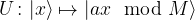
Next, we consider the function f that maps a number k to xk modulo M. As for every classical function, we can again find a quantum circuit Uf that represents this function on the level of qubits and apply it to our state to obtain the state

In his original paper [2], Shor calls this part the modular exponentiation and shows that this is actually the part of the quantum algorithm where most gates are needed (not the quantum Fourier transform).
This state has already some periodicity built into it, as xk modulo M is periodic with period r. If we could measure all the amplitudes, we could easily determine r. However, every such measurement destroys the quantum state and we have to start again, so this algorithm will not be very efficient. So again, the measurement is an issue.
Now, Shor’s idea is to solve the measurement issue by first applying (the inverse of) a quantum Fourier transform to the first register and then measure the first register (we apply the inverse of the quantum Fourier transform while other sources will state that the algorithm uses the quantum Fourier transform itself, but this is just a matter of convention as to which transformation you call the Fourier transform). The outcome s of this measurement will then give us the period!
To get an idea why this is true, let us look at a simpler case. Assume that, before applying the quantum Fourier transform, we measure the value of the second register. Let us call this value y. Then, we can write y as a power of x modulo M. Let k0 be the smallest exponent such that

Then, due to the periodicity, all values of k such that xk = y modulo M are given by

Here the index j needs to be chosen such that k0 + jr is still smaller than M. Let A denote the number of possible choices for j. Then, after the measurement, our state will have collapsed to
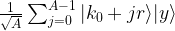
Let us now apply the inverse of the quantum Fourier transform to this state. The result will be the state

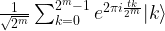
Now let us measure the first register. From the expression above, we can read off the probability P(s) to measure a certain value of s – we just have to add up the squares of all amplitudes with this value of s. This gives us

This looks complicated, but in fact this is again a geometric series with coefficient  . To see how the value of the series depends on s, let us assume for a moment that the period divides N (which is very unlikely in practice as N is a power of two, but let us assume this anyway just for the sake of argument), i.e. that N = r u with the frequency u being an integer. Thus, if s is a multiple of u, the coefficient q is equal to one (as
  ) and the geometric series sums up to A, giving probability 1 / N to measure this value. If, however, s is not a multiple of u, the value of the geometric series is

But in our case, A is of course simply equal to u, and therefore qA is equal to one. Thus the amplitude is zero! We find – note the similarity to our analysis of the Fourier transform of a periodic sequence – that P(s) is sharply peaked at multiples of  !
!
We were able to derive this result using a few simplifications – an additional measurement and the assumption that the frequency is an integer. However, as carried out by Shor in [2], a careful analysis shows that these assumptions are not needed. In fact, one can show (if you want to see all the nitty-gritty details, you could look at Shor’s paper or at my notes on GitHub that are based on an argument that I have seen first in Preskill’s lecture notes) that with reasonably high probability, the result s of the measurement will be such that

where  denotes the residual of sr modulo N. Intuitively, this means that with high probability, the residual is very small, i.e. rs is close to a multiple of N, i.e. s is close to a multiple of N / r. In other words, it shows that in fact, P(s) has peaks at multiples of N / r.
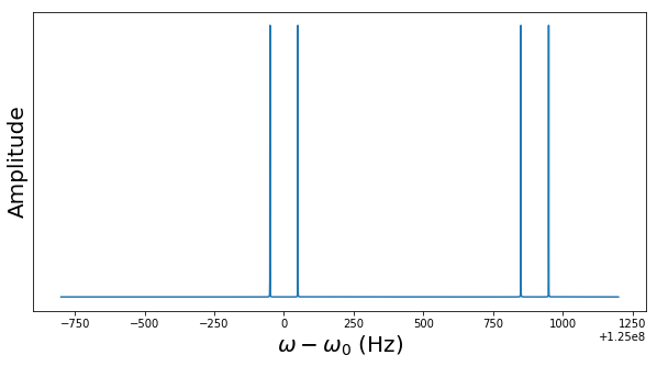
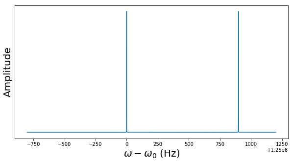
The diagram below plots the probability distribution P(s) for our example, i.e. N = 512 and r = 6 (this plot has been generated using the demo Shor.py available in my GitHub account which uses the numpy package to simulate a run of Shor’s algorithm on a classical computer)
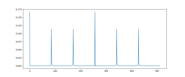
As expected, we see sharp peaks, located roughly at multiples of 512 / 6 = 85.33. So when we measure the first register, the value s will be close to a multiple of 512 / 6 with a very high probability.
So the quantum algorithm can be summarized as follows.
- Prepare a superposition
- Apply the (inverse of the) quantum Fourier transform to this state
- Measure the value of the first register and call the result s
When running the simulation during which the diagram above was created, I did in fact get a measurement at s = 427 which is very close to 5*512 / 6.
Extracting the period
So having our measurement s = 427 in our hands, how can we use this to determine the period r? We know from the considerations above that s is close to a multiple of N / r, i.e. we know that there is an integer d such that
which we can rewrite as
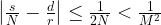
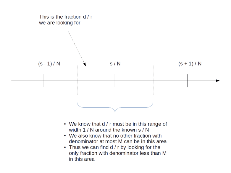
Thus we are given two rational numbers – s / N and d / r – which we know to be very close to each other. We have the first number s / N in our hands and want to determine the second number. We also know that the denominator r of the second number is smaller than M. Is this sufficient to determine d and r?
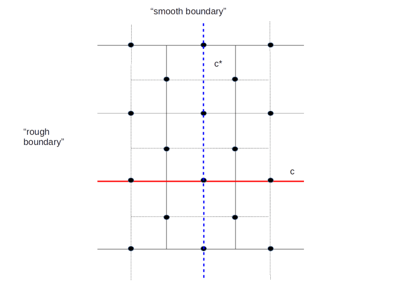
Surprisingly, the answer is “yes”. We will not go into details at this point and gloss over some of the number theory, but refer the reader to the classical reference [1] or to my notes for more details). The first good news is that two different fractions with denominators less than M need to be at least by 1 / M2 apart, so the number d / r is unique. The situation is indicated in the diagram below.
But how to find it? Luckily, the theory of continued fractions comes to the rescue. If you are not familiar with continued fractions, you can find out more in the appendix of my notes or on the very good Wikipedia page on this. Here, we will just go through the general procedure using our example at hand.
First, we write

We can do the same with 85 / 427, i.e. we can write

which will give us the decomposition
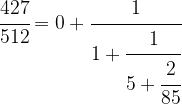
Driving this one step further, we finally obtain
This is called the continued fraction expansion of the rational number 427 / 512. More generally, for every sequence ![[a_0 ; a_1, a_2, \dots ]](https://s0.wp.com/latex.php?latex=%5Ba_0+%3B+a_1%2C+a_2%2C+%5Cdots+%5D&bg=FFFFFF&fg=000&s=0&c=20201002) , we can form the continued fraction
, we can form the continued fraction
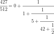
given by that sequence of coefficients, which is obviously a rational number. One can show that in fact every rational number has a representation as a continued fraction, and our calculation has shown that
![\cfrac{427}{512} = [0; 1,5,42,2]](https://s0.wp.com/latex.php?latex=%5Ccfrac%7B427%7D%7B512%7D+%3D+%5B0%3B+1%2C5%2C42%2C2%5D++&bg=FFFFFF&fg=000&s=1&c=20201002)
This sequence has five coefficients. Now given a number m, we can of course look at the sequence that we obtain by looking at the cofficients up to index m only. For instance, for m = 3, this would give us the sequence
![[0; 1,5,42]](https://s0.wp.com/latex.php?latex=%5B0%3B+1%2C5%2C42%5D++&bg=FFFFFF&fg=000&s=1&c=20201002)
The rational number represented by this sequence is

and is called the m-th convergent of the original continued fraction. We have such a convergent for every m, and thus get a (finite) series of rational numbers with the last one being the original number.
One can now show that given any rational number x, the series of m-th convergents of its continued fraction expansion has the following properties.
- The convergents are in their lowest terms
- With increasing m, the difference between x and the m-th convergent gets smaller and smaller, i.e. the convergents form an approximation of x that gets better and better
- The denominators of the convergents are increasing
So the convergents can be used to approximate the rational number x by fractions with smaller denominator – and this is exactly what we need: we wish to approximate the rational number s / N by a ratio d / r with smaller denominator which we then know to be the period. Thus we need to look at the convergents of 427 / 512. These can be easily calculated and turn out to be

The last convergent whose denominator is still smaller than M = 21 is 5 / 6, and thus we obtain r = 6. This is the period that we are looking for!
So in general, the recipe to get from the measured value s to r is to calculate the convergents of the rational number s / N and pick the denominator of the last convergent that has a denominator less than M. Again, if you want to see the exact algorithm, you can take a look at my script Shor.py.
Find the factor
We are almost done. We have run the quantum algorithm to obtain an approximate multiple of N / r. We have then applied the theory of continued fractions to derive the period r of x from this measurement. The last step – which is again a purely classical step – is now to use this to find a factor of M. This is in fact comparatively easy.
Recall that – by definition of the period – we get one if we raise x to the power of r and than reduce module M. In other words, xr minus one is a multiple of M. Now assume that we are lucky and the period r is even. Then

With a bit of elementary number theory, one can now show that this implies that the greatest common divisor gcd(xr/2-1, M) is a factor of M (unless, in fact, xr/2 is minus one modulo M, in which case the argument fails). So to get from the period to a potential factor of M, we simply calculate this greatest common divisor and check whether it divides M!
Let us do this for our case. Our period is r = 6. With x = 11, we have x3 = 1331, which is 8 module M. Thus

which is the factor of M = 21 that we were looking for.
Performance of the algorithm
In our derivation, we have ignored a few special cases which can make the algorithm fail. For instance, suppose we had not measured s = 427, but s = 341 after applying the Fourier transform. Then the corresponding approximation to 341 / 512 would have been 4 / 6. However, the continued fraction algorithm always produces a result that is in its lowest terms, i.e. it would give us not 4 / 6, but 2 / 3. Looking at this, we would infer that r = 3, which is not the correct result.
There are a few other things that can go wrong. For instance, we could find a period r which is odd, so that our step to derive a factor of M from r does not work, or we might measure an unlikely value of s.
In all these cases, we need to start over and repeat the algorithm. Fortunately, Shor could show that the probability that any of this happens is bounded from below. This bound is decreasing with larger values of M, but it is decreasing so slowly that the expected number of trials that we need grows at most logarithmically and does not destroy the overall performance of the algorithm.
Taking all these considerations into account and deriving bounds for the number of gates required to perform the quantum part of the algorithm, Shor was able to show that the number of steps to obtain a result grows at most polynomially with the number of bits that the number M has. This is obviously much better than the best classical algorithm that requires a bit less than exponential time to factor M. Thus, assuming that we are able to build a working quantum computer with the required number of gates and qubits, this algorithm would be able to factorize large numbers exponentially faster than any known classical algorithm.
Shor’s algorithm provides an example for a problem that is believed to be in the class NP (but not in P) on a classical computer, but in the class BQP on a quantum computer – this is the class of all problems that can be solved in polynomial time with a finite probability of success. However, even though factorization is generally believed not to be in P, i.e. not doable in polynomial time on classical hardware, there is not proof for that. And, even more important, it is not proved that factorization is NP-complete. Thus, Shor’s algorithm does not render every problem in NP solvable in polynomial time on a quantum computer. It does, however, still imply that all public key cryptography systems like RSA that rely on the assumption that large numbers are difficult to factor become inherently insecure once a large scale reliable quantum computer becomes available.
References
1. G.H. Hardy, E.M. Wright, An introduction to the theory of numbers, Oxford University Press, Oxford, 1975
2. P. Shor, Polynomial-Time Algorithms for Prime Factorization and Discrete Logarithms on a Quantum Computer, SIAM J.Sci.Statist.Comput. Vol. 26 Issue 5 (1997), pp 1484–1509, available as arXiv:quant-ph/9508027v2

![H = E_C[N - N_g] - E_0 \cos \delta](https://s0.wp.com/latex.php?latex=H+%3D+E_C%5BN+-+N_g%5D+-+E_0+%5Ccos+%5Cdelta++&bg=FFFFFF&fg=000&s=1&c=20201002)


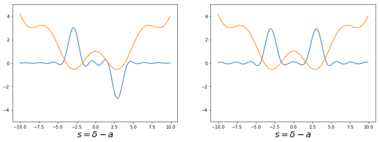

 is a state localized around the left minimum of the potential and
  is a state centered around the right minimum, whereas the first excited state is a linear combination proportional to
 in an interpretation as a qubit – and our first excited state
  are superpositions of these two states.
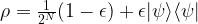
 . Here, N is the number of spins, and the factor 1/2N has been inserted to normalize the state. This density matrix describes an ensemble for which almost all molecules are in purely statistically distributed states, but a small fraction – measured by
  – of them are in a pure state. The second term in this expression is often called the deviation and denoted by
  .
.
 . Similarly, one can show that if A is an observable, described by a hermitian matrix (which, for technical reasons, we assume to be traceless), then the expectation value of A evaluated on


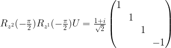
 . The matrix on the right hand side of this equation represents a two-qubit transformation known as the controlled phase gate. This gate corresponds to applying a phase gate to the second qubit, conditional on the state of the first qubit.


 .
.
 and the spin operator
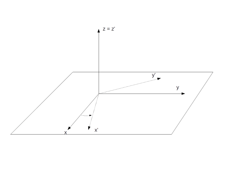
 . Geometrically, this is a rotation around the z-axis by the angle
  . Using the formula above and the fact that T commutes with the original Hamiltonian, we find that the transformed Hamiltonian is

 , we place ourselves in a frame of reference rotating with the same frequency around the z-axis. In this rotating frame, the state vector will be constant, corresponding to the fact that the new Hamiltonian vanishes. If we choose a reference frequency different from the Larmor frequency, we will observe a precession with the frequency
  .
.
![H = \omega I_z + \omega_{nut} [I_x \cos (\omega_{ref}t + \Phi_p) + I_y \sin (\omega_{ref}t + \Phi_p) ]](https://s0.wp.com/latex.php?latex=H+%3D+%5Comega+I_z+%2B+%5Comega_%7Bnut%7D+%5BI_x+%5Ccos+%28%5Comega_%7Bref%7Dt+%2B+%5CPhi_p%29+%2B+I_y+%5Csin+%28%5Comega_%7Bref%7Dt+%2B+%5CPhi_p%29+%5D++&bg=FFFFFF&fg=000&s=1&c=20201002)
![\tilde{H} = \omega_{nut} [I_x \cos \Phi_p + I_y \sin \Phi_p ]](https://s0.wp.com/latex.php?latex=%5Ctilde%7BH%7D+%3D+%5Comega_%7Bnut%7D+%5BI_x+%5Ccos+%5CPhi_p+%2B+I_y+%5Csin+%5CPhi_p+%5D++&bg=FFFFFF&fg=000&s=1&c=20201002)
 . The time evolution of this density matrix is governed by the Liouville-von Neumann equation
![i\hbar \frac{d}{dt} \rho = [H,\rho]](https://s0.wp.com/latex.php?latex=i%5Chbar+%5Cfrac%7Bd%7D%7Bdt%7D+%5Crho+%3D+%5BH%2C%5Crho%5D++&bg=FFFFFF&fg=000&s=1&c=20201002)
 is a traceless hermitian matrix. Any such matrix can be expressed as a linear combination of the Pauli matrices with real coefficients. Consequently, we can write


 (the reason for this notation will become apparent in a second) and a unit vector n.
![[a\cdot I, b \cdot I] = i \hbar (a \times b) \cdot I](https://s0.wp.com/latex.php?latex=%5Ba%5Ccdot+I%2C+b+%5Ccdot+I%5D+%3D+i+%5Chbar+%28a+%5Ctimes+b%29+%5Ccdot+I++&bg=FFFFFF&fg=000&s=1&c=20201002)
![\dot{f} = - \omega_{eff} [f \times n]](https://s0.wp.com/latex.php?latex=%5Cdot%7Bf%7D+%3D+-+%5Comega_%7Beff%7D+%5Bf+%5Ctimes+n%5D++&bg=FFFFFF&fg=000&s=1&c=20201002)
 . Therefore, according to the density matrix formalism, the expectation value of the x-component of the magnetic moment
  is
is
 and use the fact that the trace of a product of two different Pauli matrices is zero, we find that the only term that contributes to the trace is the term fx, i.e.


 , we can write this as

 . If we calculate the exponential in the Boltzmann distribution by expanding into a power series, we can therefore neglect all terms except the constant term and the term linear in

 , this changes. We have already seen that in the rotating frame, this pulse adds an additional term

 . If, for instance, we choose
  , the vector f – and thus the magnetic moment – will slowly rotate around the x-axis. If we turn off the pulse after a time

 of the first nucleus and the reference frequency, so that the value zero corresponds to
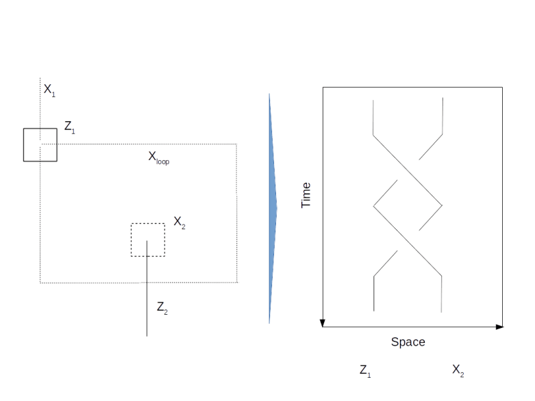
 (here and in the sequel, we assume that errors are actually corrected and not just detected to simplify our calculations) on which all stabilizers act trivially, and starting with the next round of measurements, we exclude a Zf operator from the measurements.
 . By removing
  (and adding Zf again to the set of stabilizers), we would obtain a different code space – we can think of this different code space as a deformation of the code space given by removing Zf.
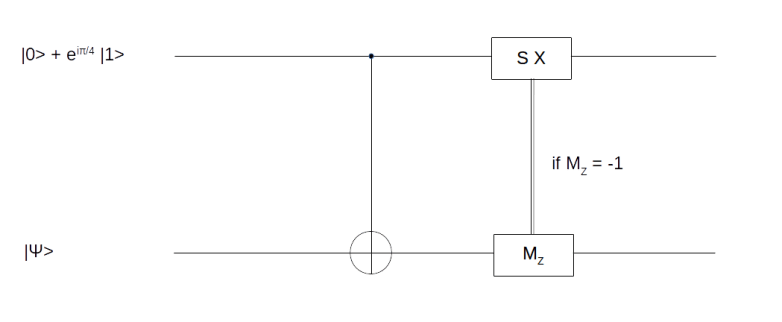


 and we are done. If not, i.e. if the measurement results in minus one, then the above formula shows that the resulting state in the first qubit will be
  . Now one can easily verify that


 between zero and one. The quantum phase estimation is designed to determine (or at least approximate) the number
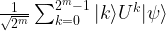
 , with binary digits ki, we can of course write Uk as
![U^k = \prod_i \big[ U^{2^i} \big]^{k_i}](https://s0.wp.com/latex.php?latex=U%5Ek+%3D+%5Cprod_i+%5Cbig%5B+U%5E%7B2%5Ei%7D+%5Cbig%5D%5E%7Bk_i%7D++&bg=FFFFFF&fg=000&s=1&c=20201002)
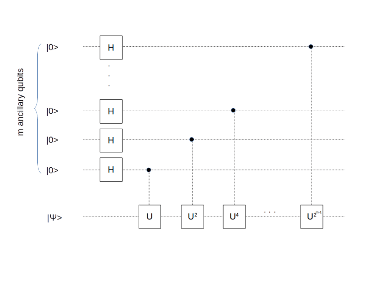
![\frac{1}{\sqrt{2^m}} \sum_{k=0}^{2^m - 1} |k \rangle U^k |\psi \rangle = \frac{1}{\sqrt{2^m}} \big[\sum_{k=0}^{2^m - 1} e^{2\pi i \varphi k} |k \rangle \big] \otimes |\psi \rangle](https://s0.wp.com/latex.php?latex=%5Cfrac%7B1%7D%7B%5Csqrt%7B2%5Em%7D%7D+%5Csum_%7Bk%3D0%7D%5E%7B2%5Em+-+1%7D+%7Ck+%5Crangle+U%5Ek+%7C%5Cpsi+%5Crangle+%3D++%5Cfrac%7B1%7D%7B%5Csqrt%7B2%5Em%7D%7D+%5Cbig%5B%5Csum_%7Bk%3D0%7D%5E%7B2%5Em+-+1%7D+e%5E%7B2%5Cpi+i+%5Cvarphi+k%7D+%7Ck+%5Crangle+%5Cbig%5D+%5Cotimes++%7C%5Cpsi+%5Crangle++&bg=FFFFFF&fg=000&s=1&c=20201002)

 ! So we can obtain t and therefore
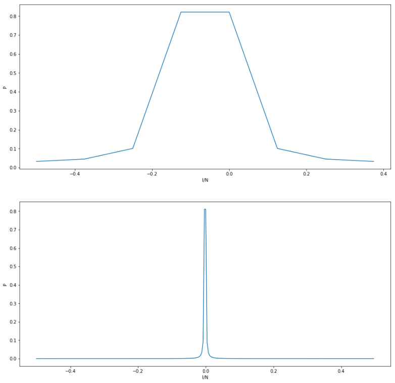
 is an integer. We can therefore use the phase estimation algorithm to obtain the period r.


 called the Pauli group. Put differently, the Pauli group consists of those linear operators on the Hilbert space that can be written as a product
 and an overall phase factor
  (we can even assume that all the
  are equal to one as
  is a multiple of
  ). Any two elements of the Pauli group either commute or anti-commute. Within this group, we now consider a finite set
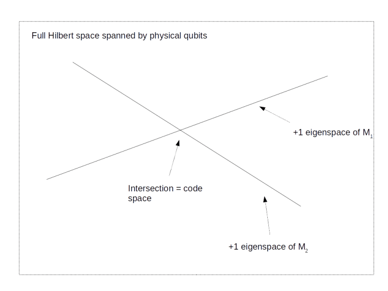
  of commuting elements and the subgroup S of the Pauli group generated by this set. This group (which is abelian as it is generated by mutually commuting elements) is called the stabilizer group. To this group, we can associate the subspace that consists of all vectors that are fixed by all elements of the group, i.e. the space
 – you might want to take a look at
 is now in the -1 eigenspace of s. Thus if we measure all elements of S, the outcome -1 for one of the measurements will tell us that an error has occurred. A similar argument shows that if the product of any two errors anti-commutes with at least one element of S, then we can also correct the error based on only the measurement results of elements in S. Mathematically speaking, the set of all elements of the Pauli group that commute with all elements of S is the centralizer of S, which in this case turns out to be equal to the normalizer N(S) of S, and a set
  of errors can be detected and corrected if and only if
 . So the elements of the Pauli group that are neither in S nor in N(S) correspond to correctable errors.
 is again fixed by all elements of S and therefore in the code space TS. Thus the elements of N(S) generate automorphisms of the code space, i.e. logical operations. It is one of the strengths of the stabilizer formalism that once we have the stabilizer group S, we can not only derive the code space and the correctable errors, but can also use group theoretic considerations to describe logical operations – this will become clearer as we study surface codes in a later post.
 will be changed to
  during transmission, where
  is the usual bit flip operator, and with probability 1-p, the transmission does not change the state. The aim is to construct an encoding of a qubit such that these errors can be detected and corrected.

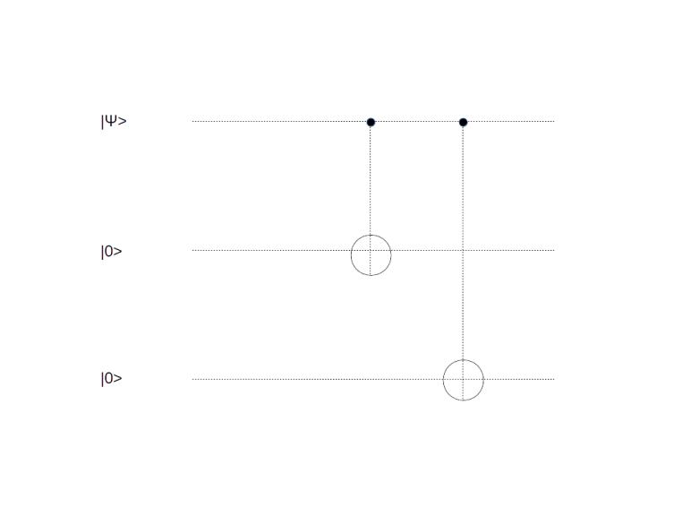
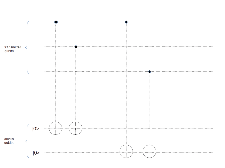
 , and no error did occur during the transmission. Then the three qubits at the top of the circuit will still be

 . Therefore both ancilla qubits will be inverted, and we obtain the state
 , so that the encoded state will be
  . When we go through the above exercise for all possible cases, we arrive at the following table that shows the transmission error and the resulting state after passing the syndrome measurement circuit.


 . In contrast to our earlier assumption that the error operator is discrete, i.e. is either applied or not applied, this operator is now continuous, depending on the parameter


 , corresponding to a logical zero and a logical one. More generally, the space C can have dimension 2n and the full Hilbert space can have dimension 2k, in which case we can encode n qubits in a larger set of k qubits (in the nine qubit code example, k = 9 and n = 1).
  that we call code words. In the case n = 1, it is common practice to denote the codewords by
  and
and  to indicate that they represent a logical qubit encoded using k physical qubits.
  like the phase flip or bit flip operators acting on the larger Hilbert space. These operators represent the impact of discretized noise and will generally move the code words out of the code space, i.e. they will rotate the code space onto different subspaces of the entire Hilbert space.
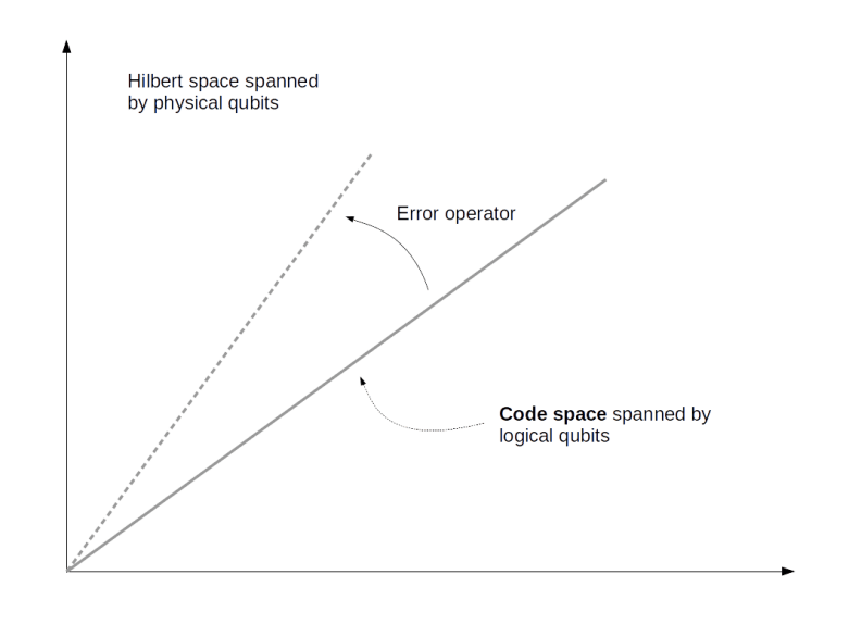
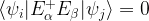
 and for all
  . Thus, even in the presence of errors, the different code words will never overlap.

 . If the matrix has full rank, the code is called non-degenerate, otherwise – as in the case of the nine qubit code – the code is called degenerate.


