In this post, I will show you how a bitcoin transaction presented in the raw format is to be interpreted and how conversely a bitcoin transaction stored in a C++ (and later Python) object can be converted into a hexadecimal representation (a process called serialization). Ultimately, the goal of this and subsequent posts will be to create a bitcoin transaction from scratch in Python, to sign it and to publish it in a bitcoin network, without using any of the available bitcoin libraries.
The subject of serialization and deserialization in the bitcoin protocol is a bit tricky. At the end of the day, the truth is hidden in the reference implementation somewhere (so time to get the code from the GitHub repository if you have not done so yet). I have to admit that when I first started to work with that code, I found it not exactly easy to understand, given that it has been a few years (well, somewhere around 20 years to be precise) since I last worked with templates in C++. Still, the idea of this post is to get to the bottom of it, and so I will walk you through the most relevant pieces of the source code. But be warned – this will not be an easy read and a bit lengthy. Alternatively, you can also skip directly to the end where the result is again summarized and ignore the details.
The first thing that we need is access to a raw (serialized) bitcoin transaction. This can be obtained from blockchain.info using the following code snippet.
import requests

def get_raw_transaction(txid="ed70b8c66a4b064cfe992a097b3406fa81ff09641fe55a709e4266167ef47891"):
    url = 'https://blockchain.info/en/tx/' + txid + '?format=hex'
    r = requests.get(url)
    return r.text
If you print the result, you should get
0200000003620f7bc1087b0111f76978ef747001e3ae0a12f254cbfb858f
028f891c40e5f6010000006a47304402207f5dfc2f7f7329b7cc731df605
c83aa6f48ec2218495324bb4ab43376f313b840220020c769655e4bfcc54
e55104f6adc723867d9d819266d27e755e098f646f689d0121038c2d1cbe
4d731c69e67d16c52682e01cb70b046ead63e90bf793f52f541dafbdfeff
fffff15fe7d9e0815853738ce47deadee69339e027a1dfcfb6fa887cce3a
72626e7b010000006a47304402203202e6c640c063989623fc782ac1c9dc
3c6fcaed996d852ec876749ba63db63b02207ef86e262ad4b4bc9cebfadb
609f52c35b0105e15d58a5ecbecc5e536d3a8cd8012103dc526ca188418a
b128d998bf80942d66f1b3be585d0c89bd61c533bddbdaa729feffffff84
e6431db86833897bab333d844486c183dd01e69862edea442e480c2d8cb5
49010000006a47304402200320bc83f35ceab4a7ef0f8181eedb5f54e3f6
17626826cc49c8c86efc9be0b302203705889d6aed50f716b81b0f3f5769
d72d1b8a6b59d1b0b73bcf94245c283b8001210263591c21ce8ee0d96a61
7108d7c278e2e715ac6d8afd3fcd158bee472c590068feffffff02ca780a
00000000001976a914811fb695e46e2386501bcd70e5c869fe6c0bb33988
ac10f59600000000001976a9140f2408a811f6d24ab1833924d98d884c44
ecee8888ac6fce0700
Having that, we can now start to go through this byte by byte – you might even want to print that string and strike out the bytes as we go. To understand how serialization works in the reference implementation, we will have to study the the header file serialize.h containing boilerplate code to support serialization. In addition, each individual data type contains specific serialization code. It is useful to compare our results with the human readable description of the transaction at blockchain.info.
To understand how the mechanism works, let us start at the function getrawtransaction in rpc/rawtransaction.cpp which is implementing the corresponding RPC call. This function ends up calling TxToUniv in core_write.cpp and finally EncodeHexTx in the same file. Here an instance of the class CDataStream is created which is defined in streams.h. For that class, the operator << is overwritten so that the function Serialize is invoked. Templates for this method are declared in serialize.h and will tell us how the individual data types are serialized in each individual case for the elementary data types and sets, vectors etc.. All composite classes need to implement their own Serialize method to fit into this scheme.
For a transaction, the method CTransaction::Serialize is defined in primitives/transaction.h and delegates the call to the function SerializeTransaction in the same file.
template
inline void SerializeTransaction(const TxType& tx, Stream& s) {
    const bool fAllowWitness = !(s.GetVersion() & SERIALIZE_TRANSACTION_NO_WITNESS);

    s << tx.nVersion;
    unsigned char flags = 0;
    // Consistency check
    if (fAllowWitness) {
        /* Check whether witnesses need to be serialized. */
        if (tx.HasWitness()) {
            flags |= 1;
        }
    }
    if (flags) {
        /* Use extended format in case witnesses are to be serialized. */
        std::vector vinDummy;
        s << vinDummy;
        s << flags;
    }
    s << tx.vin;
    s << tx.vout;
    if (flags & 1) {
        for (size_t i = 0; i < tx.vin.size(); i++) {
            s << tx.vin[i].scriptWitness.stack;
        }
    }
    s << tx.nLockTime;
}
Throughout this post, we will ignore the extended format that relates to the segregated witness feature and restrict ourselves to the standard format, i.e. to the case that the flag fAllowWitness above is false.
We see that the first four bytes are the version number, which is 2 in this case. Note that little endian encoding is used, i.e. the first byte is the least significant byte. So the version number 2 corresponds to the string
02000000
Next, the transaction inputs and transaction outputs are serialized. These are vectors, and the mechanism for serializing vectors becomes apparent in serialize.h.
template
void Serialize_impl(Stream& os, const std::vector& v, const V&)
{
    WriteCompactSize(os, v.size());
    for (typename std::vector::const_iterator vi = v.begin(); vi != v.end(); ++vi)
        ::Serialize(os, (*vi));
}

template
inline void Serialize(Stream& os, const std::vector& v)
{
    Serialize_impl(os, v, T());
}
We see that to serialize a vector, we first serialize the length of the vector, i.e. the number of elements, and then call the serialization method on each of the individual items. The length is serialized in a compact format called a varInt which stores a number in 1 – 9 bytes, depending on its size. In this case, one byte is sufficient – this is the byte 03 after the version number. Thus we can conclude that the transaction has three transaction inputs.
To understand the next bytes, we need to look at the method CTxIn::SerializeOp.
template
inline void SerializationOp(Stream& s, Operation ser_action) {
    READWRITE(prevout);
    READWRITE(scriptSig);
    READWRITE(nSequence);
}
This is not very surprising – we see that the spent transaction output, the signature script and the sequence number are serialized in that order. The spent transaction prevout is an instance of COutPoint which has its own serialization method. First, the transaction ID of the previous transaction is serialized according to the method base_blob::Serialize defined in uint256.h. This will produce the hexadecimal representation in little endian encoding, so that we have to reverse the order bytewise to obtain the transaction ID.
So in our example, the ID of the previous transaction is encoded in the part starting with 620f7b… in the first line and ending (a transaction ID has always 256 bit, i.e. 32 bytes, i.e. 64 characters) with the bytes …1c40e5f6 early in the second line. To get the real transaction ID, we have to revert this byte for byte, i.e. the transaction ID is
f6e5401c898f028f85fbcb54f2120aaee3017074ef7869f711017b08c17b0f62
The next four bytes still belong to the spent transaction and encode the index of the spent output in the list of outputs of the previous transaction. In this case this is 1, again encoded in little endian byte order, i.e. as 01000000. Thus we have now covered and understood the following part of the hex representation.
0200000003620f7bc1087b0111f76978ef747001e3ae0a12f254cbfb858f
028f891c40e5f601000000
Going back to the serialization method of the class CTxIn, we now see that the next few bytes are the signature script. The format of the signature script is complicated and will be covered in a separate post. For today, we simply take this as a hexadecimal string. In our case, this string starts with 6a473044 …. in the second line and ends with … 541dafbd close to the end of line five.
Finally, the last two bytes in line five and the first two bytes in line six are the sequence number in little endian byte order.
We are now done with the first transaction input. There are two more transaction inputs that follow the same pattern, the last one ends again with the sequence number close to the end of line 15.
Now we move on to the transaction outputs. Again, as this is a vector, the first byte (02) is the number of outputs. Each output is then serialized according to the respective method of the class TxOut.
template
inline void SerializationOp(Stream& s, Operation ser_action) {
    READWRITE(nValue);
    READWRITE(scriptPubKey);
}
The first element is the value, which is an instance of the class CAmount. Again, we can look up the serialization method of this class in amount.h and find that this is simply a 64 bit integer, so its serialization method is covered by the templates in serialize.h and results simply in eight bytes in little endian order:
ca780a0000000000
If we reorder and decode this, we obtain 686282 Satoshi, i.e. 0.0686282 bitcoin. The next object that is serialized is the public key script. Again, we leave the details to a later post, but remark that (which is also true for the signature script) the first byte is the length of the remaining part of the script in bytes, so that we can figure out that the script is composed of the 0x19 = 25 bytes
76a914811fb695e46e2386501bcd70e5c869fe6c0bb33988ac
For the second output, the pattern repeats itself. We have the amount and the public key script
76a9140f2408a811f6d24ab1833924d98d884c44ecee8888ac
of the second output.
Finally, there are four bytes left: 6fce0700. Going back to SerializeTransaction, we identify this as the lock time 0x7ce6f ( 511599 in decimal notation).
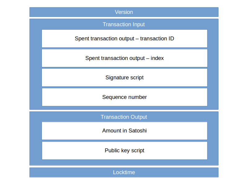
After going through all these details, it is time to summarize our findings. A bitcoin transaction is encoded as a hexadecimal string as follows.
- The version number (4 bytes, little endian)
- The number of transaction inputs
- For each transaction input:
- the ID of the previous transaction (reversed)
- the index of the spent transaction output in the previous transaction (4 bytes, little endian)
- the length of the signature script
- the signature script
- the sequence number (4 bytes, little endian)
- The number of transaction outputs
- For each transaction output:
- the amount (eight bytes, little endian encoding) in Satoshi
- the length of the public key script
- the public key script
- the locktime (four bytes, little endian)
In my GitHub account, you will find a Python script Transaction.py that retrieves our sample transaction from the blockchain.info site and prints out all the information line by line. To run it, clone the repository using
$ git clone https://github.com/christianb93/bitcoin.git ; cd bitcoin
and then run the script
$ python Transaction.py
The script uses a few modules in the package btc, namely txn.py and serialize.py that essentially implement the serialization and deserialization routines discussed in this post.
That is it for today. In the next posts, I will start to look at a topic that we have more or less consequently ignored or oversimplified so far: scripts in the bitcoin world.


 .
. is the strength of the connection between the units i and j. We assume that no neuron is connected to ifself, i.e. that
  , and that the matrix of weights is symmetric, i.e. that
  .
.

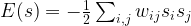
 . Let
. Let


 and the activation of unit i is never negative, this implies that during the upgrade process, the energy function will always increase or stay the same. Thus the state will settle in a local minimum of the energy function.
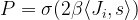

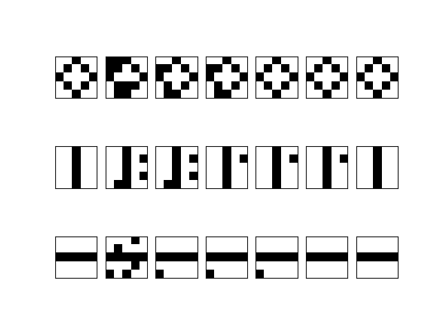
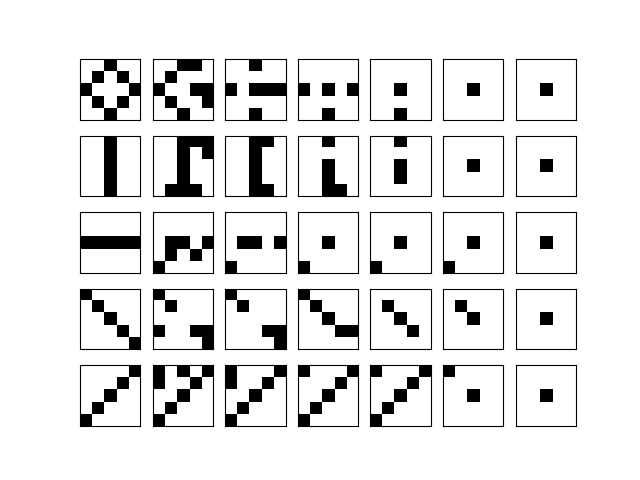
 is close to infinity. If the activation of unit i is positive, the probability will be very close to one. The Gibbs sampling rule will then almost certainly set the spin to +1. If the activation is negative, the probability will be zero, and we will set the spin to -1. Thus the update role of a Hopfield network corresponds to the Gibbs sampling step for an Ising model at temperature zero.
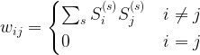
 are the states that the network should remember (in a later post in this series, we will see that this rule can be obtained as the low temperature limit of a training algorithm called contrastive divergence that is used to train a certain class of Boltzmann machines).
 and
and  have the same sign, i.e. are in the same state. This corresponds to a rule known as Hebbian learning rule that has been postulated as a principle of learning by D. Hebb and basically states that during learning, connections between neurons are enforced if these neurons fire together (

 .
. .
.

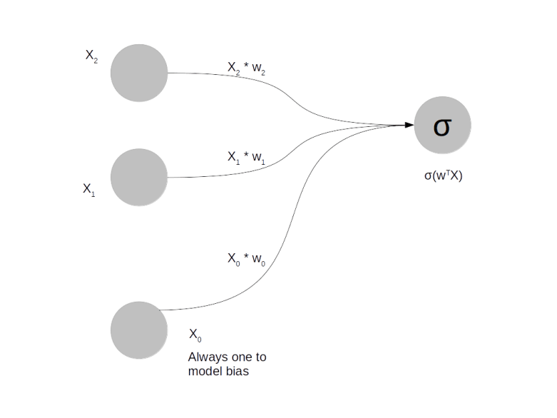
 , as follows.
 is a function called the activation function and
  is the vector that is formed by
  and
and  . There are a few standard choices for the activation function, a common one being the

 . Even if we cannot find an analytic expression for this, we can try to approximate it. Your first idea might be “Riemann sums”, but it turns out that this is not a good idea, as our function lives in the space of all weights which has a very high dimension. Instead, we will use an approach called Monte Carlo integration where we represent the integral as an expectation value, draw a sample and approximate the expectation value by the sample average. This is where stochastical methods like Markov chains will come into play. And finally we will see that the behaviour of our network during training has some striking analogies with the behaviour of certain physical systems like solids exposed to a magnetic field at low temperatures, which are described by a model called the Ising model, and learn how techniques that physicists have developed for this type of problems apply to neuronal networks.


 and
and  , the coordinates of their sum
  can be determined as follows.
 and
and  with
with
