Hopfield networks: practice

After having discussed Hopfield networks from a more theoretical point of view, let us now see how we can implement a Hopfield network in Python.

First let us take a look at the data structures. We will store the weights and the state of the units in a class HopfieldNetwork. The weights are stored in a matrix, the states in an array.

class HopfieldNetwork:

    #
    # Initialize a Hopfield network with N
    # neurons
    #
    def __init__(self, N):
        self.N = N
        self.W = np.zeros((N,N))
        self.s = np.zeros((N,1))

Next we write a method for the update rule. In a matrix notation, the activation of unit i is given as the dot product of the current state and the i-th row of the weight matrix (or the i-th column, as the matrix is symmetric). Therefore we can use the following update function.

#
# Run one simulation step
#
def runStep(self):
    i = np.random.randint(0,self.N)
    a = np.matmul(self.W[i,:], self.s)
    if a < 0:
        self.s[i] = -1
    else:
        self.s[i] = 1

Finally, there is the Hebbian learning rule. If we store the sample set in a matrix S such that each row corresponds to one sample, the learning rule is equivalent to

Thus we can again use the matrix multiplication from the numpy package, and our learning rule is simply

def train(self, S):
    self.W = np.matmul(S.transpose(), S)

Now we need some pattern to train our network. For the sake of demonstration, let us use a small network with 5 x 5 units, each of them representing a pixel in a grayscale 5 x 5 image. For this post, I have hardcoded five simple patterns, but we could of course use any other training set.

To illustrate how the Hopfield network operates, we can now use the method train to train the network on a few of these patterns that we call memories. We then take these memories and randomly flip a few bits in each of them, in other words we simulate random errors in the pattern. We then place the network in these states and run the update rule several times. If you want to try this yourself, get the script Hopfield.py from my GitHub repository.

 
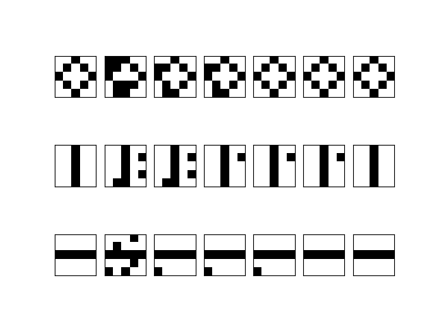
The image above shows the result of this exercise. Here we have stored three memories – the first column of images – in the network. The second image in each row then shows the distorted versions of these patterns after flipping five bits randomly. The next images in each row show the state of the network after 20, 40, 60, 80 and 100 iterations of the update rule. We see that in this case, all errors could be removed and the network did in fact converge to the original image.

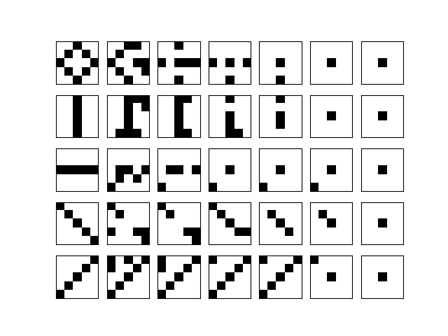
However, the situation becomes worse if we try to store more memories. The next image shows the outcome of a simulation with the same basic parameters, but five instead of three memories.

We clearly see that not a single one of the distorted patterns converges to the original image. Apparently, we have exceeded the capacity of the network. In his paper, Hopfield – based on theoretical considerations and simulations – argues that the network can only store approximately patterns, where N is the number of units. In our case, with 25 units, this would be approximately 3 to 4 patterns.

If we exceed this limit, we seem to create local minima of the energy that do not correspond to any of the stored patterns. This problem is known as the problem of spurious minima which can also occur if we stay below the maximum capacity – if you do several runs with three memories, you will find that also in this case, spurious minima can occur.

The update rule of the Hopfield network is deterministic, its energy can never increase. Thus if the system moves into one of those local minima, it can never escape again and gets stuck. An Ising model at a finite, non-zero temperature behaves differently. As the update rule is stochastic, it is possible that the system moves away from a local minimum in a Gibbs sampling step, and therefore has the chance to escape from a spurious minimum. This is one of the reasons why researchers have tried to come up with stochastic versions of the Hopfield network. One of these stochastic versions is the Boltzmann network, and we will start to look at its theoretical foundations in the next post in this series.