Until the nineties of the last century, quantum computing seemed to be an interesting theoretical possibility, but it was far from clear whether it could be useful to tackle computationally hard problems with high relevance for actual complications. This changed dramatically in 1994, when the mathematician P. Shor announced a quantum algorithm that could efficiently solve one of the most intriguing problems in applied mathematics – factoring large numbers into their constituent primes, which, for instance, can be used to break commonly used public key cryptography schemes like RSA.
Shor’s algorithm is significantly more complicated than the quantum algorithms that we have studied so far, so we start with a short overview and then look at the individual pieces in more detail.
Given a number M that we want to factorize, the first part of Shor’s algorithm is to find a number x which has no common divisor with M so that it is a unit modulo M. In practice, we can just guess some x and compute the greatest common divisor gcd(x,M) – if this is not one, we have found a factor of M and are done, if this is one, we have the number x that we need. This step can still be done efficiently on a classical computer and does not require a quantum computer.
The next part of the algorithm now uses a quantum algorithm to determine the period of x. The period is the smallest non-zero number r such that
The core of this step is the quantum algorithm that we will study below. However, the quantum algorithm does not exactly return the number r, but it returns a number s which is close to a multiple of  , where N is a power of two. Getting r out of this information is again a classical step that uses the theory of continued fractions. The number N that appears here is N = 2n where n is the number of qubits that the quantum part requires, and needs to be chosen such that M2 can be represented with n bits.
Finally, the third part of the algorithm uses the period r to find a factor of M, which is again done classically using elementary number theory. Thus the overall layout of the algorithm is as follows.
- Find the smallest number n (the number of qubits that we will need) such that
 and a number
  such that gcd(x,M) = 1
- Use the quantum part of the algorithm to find a number s which is approximately an integer multiple of N / r
- Use the theory of continued fractions to extract the period r from this information
- Use the period to find a factor of M
We will know look at each of these steps in turn (yes, this is going to be a bit of a lengthy post). To make this more tangible, we use a real example and assume that we wanted to factor the number M = 21. This is of course a toy example, but it allows us to simulate and visualize the procedure efficiently on a classical computer.
Determine n and x
The first step is easy. First, we need to determine the number n of qubits that we need. As mentioned above, this is simply the bit length of M2. In our case, M2 = 441, and the next power of two is 512 = 29, so we need n = 9 qubits.
The next step is to find the number x. This can easily be done by just randomly picking some x and checking that is has no common prime factor with M. In our example, let us choose x = 11 (which is a prime number, but this is just by accident and not needed). It is important to choose this rather randomly, as the algorithm might fail in some rare instances and we need to start over, but this only makes sense if we do not pick the same choice again for our second trial.
The quantum part of the algorithm
Now the quantum part of the algorithm starts. We want to calculate the period of x = 11, i.e. the smallest number r such that xr – 1 is a multiple of M = 21.
Of course, as our numbers are small, we could easily calculate the period classically by taking successive powers of 11 and reducing modulo 21, and this would quickly tell us that the period is 6. This, however, is no longer feasible with larger numbers, and this is where our quantum algorithm comes into play.
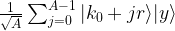
The algorithm uses two quantum registers. The first register has n qubits, the second can have less, in fact any number of qubits will do as long as we can store all numbers up to M in it, i.e. the bit length of M will suffice. Initially, we bring the system into the superposition

which we can for instance do by starting with the state with all qubits being zero and then applying the Hadamard-Walsh transformation to the first register.
Next, we consider the function f that maps a number k to xk modulo M. As for every classical function, we can again find a quantum circuit Uf that represents this function on the level of qubits and apply it to our state to obtain the state

In his original paper [2], Shor calls this part the modular exponentiation and shows that this is actually the part of the quantum algorithm where most gates are needed (not the quantum Fourier transform).
This state has already some periodicity built into it, as xk modulo M is periodic with period r. If we could measure all the amplitudes, we could easily determine r. However, every such measurement destroys the quantum state and we have to start again, so this algorithm will not be very efficient. So again, the measurement is an issue.
Now, Shor’s idea is to solve the measurement issue by first applying (the inverse of) a quantum Fourier transform to the first register and then measure the first register (we apply the inverse of the quantum Fourier transform while other sources will state that the algorithm uses the quantum Fourier transform itself, but this is just a matter of convention as to which transformation you call the Fourier transform). The outcome s of this measurement will then give us the period!
To get an idea why this is true, let us look at a simpler case. Assume that, before applying the quantum Fourier transform, we measure the value of the second register. Let us call this value y. Then, we can write y as a power of x modulo M. Let k0 be the smallest exponent such that

Then, due to the periodicity, all values of k such that xk = y modulo M are given by

Here the index j needs to be chosen such that k0 + jr is still smaller than M. Let A denote the number of possible choices for j. Then, after the measurement, our state will have collapsed to
Let us now apply the inverse of the quantum Fourier transform to this state. The result will be the state

Now let us measure the first register. From the expression above, we can read off the probability P(s) to measure a certain value of s – we just have to add up the squares of all amplitudes with this value of s. This gives us

This looks complicated, but in fact this is again a geometric series with coefficient  . To see how the value of the series depends on s, let us assume for a moment that the period divides N (which is very unlikely in practice as N is a power of two, but let us assume this anyway just for the sake of argument), i.e. that N = r u with the frequency u being an integer. Thus, if s is a multiple of u, the coefficient q is equal to one (as
  ) and the geometric series sums up to A, giving probability 1 / N to measure this value. If, however, s is not a multiple of u, the value of the geometric series is

But in our case, A is of course simply equal to u, and therefore qA is equal to one. Thus the amplitude is zero! We find – note the similarity to our analysis of the Fourier transform of a periodic sequence – that P(s) is sharply peaked at multiples of  !
!
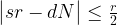
We were able to derive this result using a few simplifications – an additional measurement and the assumption that the frequency is an integer. However, as carried out by Shor in [2], a careful analysis shows that these assumptions are not needed. In fact, one can show (if you want to see all the nitty-gritty details, you could look at Shor’s paper or at my notes on GitHub that are based on an argument that I have seen first in Preskill’s lecture notes) that with reasonably high probability, the result s of the measurement will be such that

where  denotes the residual of sr modulo N. Intuitively, this means that with high probability, the residual is very small, i.e. rs is close to a multiple of N, i.e. s is close to a multiple of N / r. In other words, it shows that in fact, P(s) has peaks at multiples of N / r.
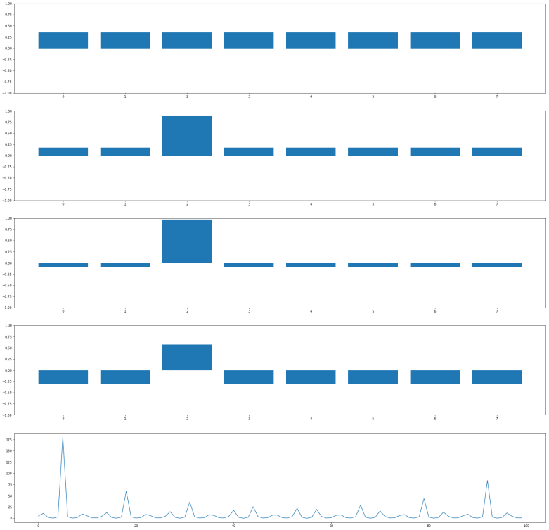
The diagram below plots the probability distribution P(s) for our example, i.e. N = 512 and r = 6 (this plot has been generated using the demo Shor.py available in my GitHub account which uses the numpy package to simulate a run of Shor’s algorithm on a classical computer)
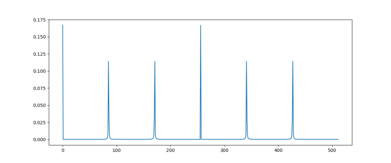
As expected, we see sharp peaks, located roughly at multiples of 512 / 6 = 85.33. So when we measure the first register, the value s will be close to a multiple of 512 / 6 with a very high probability.
So the quantum algorithm can be summarized as follows.
- Prepare a superposition
- Apply the (inverse of the) quantum Fourier transform to this state
- Measure the value of the first register and call the result s
When running the simulation during which the diagram above was created, I did in fact get a measurement at s = 427 which is very close to 5*512 / 6.
Extracting the period
So having our measurement s = 427 in our hands, how can we use this to determine the period r? We know from the considerations above that s is close to a multiple of N / r, i.e. we know that there is an integer d such that
which we can rewrite as
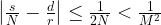
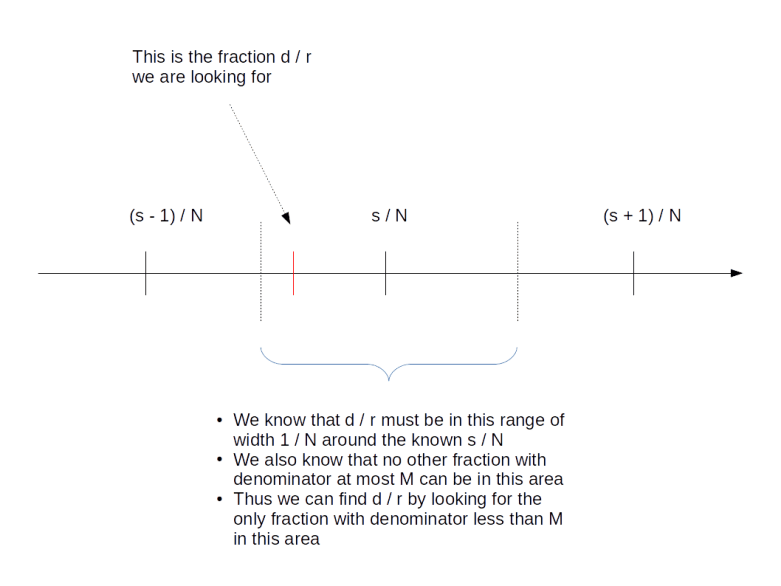
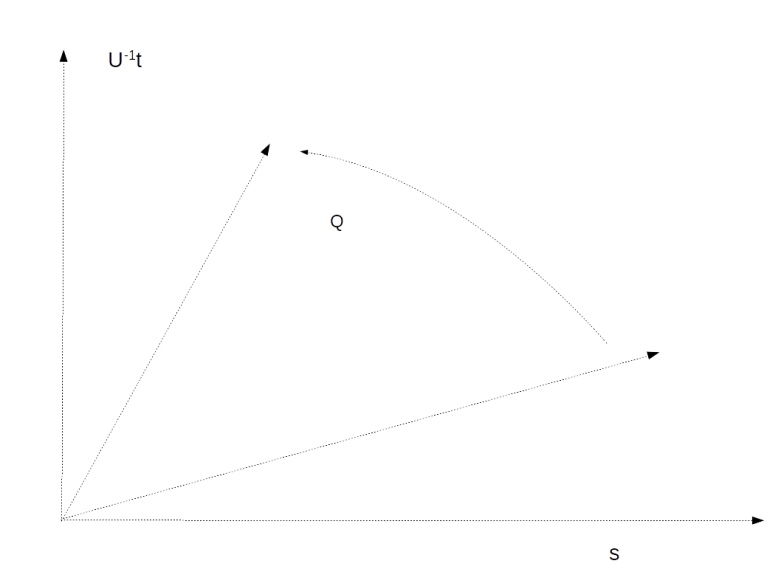
Thus we are given two rational numbers – s / N and d / r – which we know to be very close to each other. We have the first number s / N in our hands and want to determine the second number. We also know that the denominator r of the second number is smaller than M. Is this sufficient to determine d and r?
Surprisingly, the answer is “yes”. We will not go into details at this point and gloss over some of the number theory, but refer the reader to the classical reference [1] or to my notes for more details). The first good news is that two different fractions with denominators less than M need to be at least by 1 / M2 apart, so the number d / r is unique. The situation is indicated in the diagram below.
But how to find it? Luckily, the theory of continued fractions comes to the rescue. If you are not familiar with continued fractions, you can find out more in the appendix of my notes or on the very good Wikipedia page on this. Here, we will just go through the general procedure using our example at hand.
First, we write

We can do the same with 85 / 427, i.e. we can write

which will give us the decomposition
Driving this one step further, we finally obtain
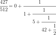
This is called the continued fraction expansion of the rational number 427 / 512. More generally, for every sequence ![[a_0 ; a_1, a_2, \dots ]](https://s0.wp.com/latex.php?latex=%5Ba_0+%3B+a_1%2C+a_2%2C+%5Cdots+%5D&bg=FFFFFF&fg=000&s=0&c=20201002) , we can form the continued fraction
, we can form the continued fraction
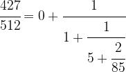
given by that sequence of coefficients, which is obviously a rational number. One can show that in fact every rational number has a representation as a continued fraction, and our calculation has shown that
![\cfrac{427}{512} = [0; 1,5,42,2]](https://s0.wp.com/latex.php?latex=%5Ccfrac%7B427%7D%7B512%7D+%3D+%5B0%3B+1%2C5%2C42%2C2%5D++&bg=FFFFFF&fg=000&s=1&c=20201002)
This sequence has five coefficients. Now given a number m, we can of course look at the sequence that we obtain by looking at the cofficients up to index m only. For instance, for m = 3, this would give us the sequence
![[0; 1,5,42]](https://s0.wp.com/latex.php?latex=%5B0%3B+1%2C5%2C42%5D++&bg=FFFFFF&fg=000&s=1&c=20201002)
The rational number represented by this sequence is

and is called the m-th convergent of the original continued fraction. We have such a convergent for every m, and thus get a (finite) series of rational numbers with the last one being the original number.
One can now show that given any rational number x, the series of m-th convergents of its continued fraction expansion has the following properties.
- The convergents are in their lowest terms
- With increasing m, the difference between x and the m-th convergent gets smaller and smaller, i.e. the convergents form an approximation of x that gets better and better
- The denominators of the convergents are increasing
So the convergents can be used to approximate the rational number x by fractions with smaller denominator – and this is exactly what we need: we wish to approximate the rational number s / N by a ratio d / r with smaller denominator which we then know to be the period. Thus we need to look at the convergents of 427 / 512. These can be easily calculated and turn out to be

The last convergent whose denominator is still smaller than M = 21 is 5 / 6, and thus we obtain r = 6. This is the period that we are looking for!
So in general, the recipe to get from the measured value s to r is to calculate the convergents of the rational number s / N and pick the denominator of the last convergent that has a denominator less than M. Again, if you want to see the exact algorithm, you can take a look at my script Shor.py.
Find the factor
We are almost done. We have run the quantum algorithm to obtain an approximate multiple of N / r. We have then applied the theory of continued fractions to derive the period r of x from this measurement. The last step – which is again a purely classical step – is now to use this to find a factor of M. This is in fact comparatively easy.
Recall that – by definition of the period – we get one if we raise x to the power of r and than reduce module M. In other words, xr minus one is a multiple of M. Now assume that we are lucky and the period r is even. Then

With a bit of elementary number theory, one can now show that this implies that the greatest common divisor gcd(xr/2-1, M) is a factor of M (unless, in fact, xr/2 is minus one modulo M, in which case the argument fails). So to get from the period to a potential factor of M, we simply calculate this greatest common divisor and check whether it divides M!
Let us do this for our case. Our period is r = 6. With x = 11, we have x3 = 1331, which is 8 module M. Thus

which is the factor of M = 21 that we were looking for.
Performance of the algorithm
In our derivation, we have ignored a few special cases which can make the algorithm fail. For instance, suppose we had not measured s = 427, but s = 341 after applying the Fourier transform. Then the corresponding approximation to 341 / 512 would have been 4 / 6. However, the continued fraction algorithm always produces a result that is in its lowest terms, i.e. it would give us not 4 / 6, but 2 / 3. Looking at this, we would infer that r = 3, which is not the correct result.
There are a few other things that can go wrong. For instance, we could find a period r which is odd, so that our step to derive a factor of M from r does not work, or we might measure an unlikely value of s.
In all these cases, we need to start over and repeat the algorithm. Fortunately, Shor could show that the probability that any of this happens is bounded from below. This bound is decreasing with larger values of M, but it is decreasing so slowly that the expected number of trials that we need grows at most logarithmically and does not destroy the overall performance of the algorithm.
Taking all these considerations into account and deriving bounds for the number of gates required to perform the quantum part of the algorithm, Shor was able to show that the number of steps to obtain a result grows at most polynomially with the number of bits that the number M has. This is obviously much better than the best classical algorithm that requires a bit less than exponential time to factor M. Thus, assuming that we are able to build a working quantum computer with the required number of gates and qubits, this algorithm would be able to factorize large numbers exponentially faster than any known classical algorithm.
Shor’s algorithm provides an example for a problem that is believed to be in the class NP (but not in P) on a classical computer, but in the class BQP on a quantum computer – this is the class of all problems that can be solved in polynomial time with a finite probability of success. However, even though factorization is generally believed not to be in P, i.e. not doable in polynomial time on classical hardware, there is not proof for that. And, even more important, it is not proved that factorization is NP-complete. Thus, Shor’s algorithm does not render every problem in NP solvable in polynomial time on a quantum computer. It does, however, still imply that all public key cryptography systems like RSA that rely on the assumption that large numbers are difficult to factor become inherently insecure once a large scale reliable quantum computer becomes available.
References
1. G.H. Hardy, E.M. Wright, An introduction to the theory of numbers, Oxford University Press, Oxford, 1975
2. P. Shor, Polynomial-Time Algorithms for Prime Factorization and Discrete Logarithms on a Quantum Computer, SIAM J.Sci.Statist.Comput. Vol. 26 Issue 5 (1997), pp 1484–1509, available as arXiv:quant-ph/9508027v2


 that is zero on all but one elements. The task is to locate the element x0 for which P(x0) is true.
 of an n-qubit system to obtain a superposition of all basis states. Then, we iteratively apply the following sequence of operations.
 to
to  .
. along the diagonal, with N = 2n, and
  away from the diagonal. In terms of basis vectors, the mapping is given by

 is the average across the amplitudes
  . Thus geometrically, the operation D performs an inversion around the average. Grover shows that this operation can be written as minus a Hadamard-Walsh operation followed by the operation that flips the sign for
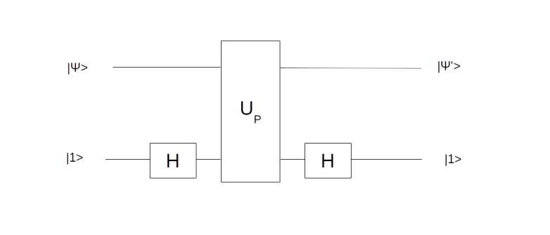

 and it will change the amplitude of this vector to – 0.35. This will change the average amplitude to a value slightly below 0.35. If we now perform the inversion around the average, the amplitudes of all basis vectors different from
  , and that doubling the number of iterations does in general lead to a less optimal result.
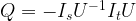
 . Applying the operation Q n times will then approximately result in a superposition of the form
 is close to a multiple of
  , then one application of U will take our state to a state very close to t.
 where x0 is the solution to the search problem. Thus the operation It is the conditional phase shift that we have denoted by S earlier. In addition, Grover shows in


 in this case, we also recover the result that the optimal number of iterations is
  applications of the transformation UP. Whether this is better than the classical algorithm does of course depend on the efficiency with which we can implement this with quantum gates. If applying UP requires O(N) operations, the advantage of the algorithm is lost. Thus the algorithm only provides a significant speedup if the operation UP can be implemented efficiently and there is no additional structure that a classical algorithm could exploit.


 , in practice this could be weights, bias terms or any other parameters. To simplify things a bit, we will also assume that the latent variable is finite. Our aim is to maximize the log likelihood, which we can – under these assumptions – express as follows.
 . For that purpose, we introduce a term that is traditionally called Q and defined as follows (all this is a bit abstract, but will become clearer later when we do an example):
![Q(\Theta'; \Theta) = E \left[ \ln P(x,z | \Theta') | x, \Theta \right]](https://s0.wp.com/latex.php?latex=Q%28%5CTheta%27%3B+%5CTheta%29+%3D+E+%5Cleft%5B++%5Cln+P%28x%2Cz+%7C+%5CTheta%27%29++%7C+x%2C+%5CTheta+%5Cright%5D++&bg=FFFFFF&fg=000&s=1&c=20201002)
 of z. Thus the right hand side is, spelled out
![E \left[ \ln P(x,z | \Theta') | x, \Theta \right] = \sum_z \ln P(x,z | \Theta') P(z | x, \Theta)](https://s0.wp.com/latex.php?latex=E+%5Cleft%5B++%5Cln+P%28x%2Cz+%7C+%5CTheta%27%29++%7C+x%2C+%5CTheta+%5Cright%5D+%3D+%5Csum_z+%5Cln+P%28x%2Cz+%7C+%5CTheta%27%29+P%28z+%7C+x%2C+%5CTheta%29++&bg=FFFFFF&fg=000&s=1&c=20201002)
 of parameters such that when passing from
  to
to  , the value of Q does not decrease, i.e.

 is maximized. This part of the algorithm is therefore called the maximization step. Then we start over, using
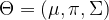


 and
and  . Using this notation, we can now write down the result of calculating the Q function:
 . For a fixed
  and
and  , and we can now try to maximize this function with respect to these parameters. This calculation is not difficult, but again a bit tiresome (and requires the use of Lagrangian multipliers as there is a constraint on the
  ), and I again refer to


 , the covariance matrices
  and the means
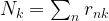
  – which could, for instance, be chosen randomly. Then, we calculate the responsibilities as above – essentially, this is the expectation step, as it amounts to finding Q.
 of points in some euclidian space and a number K of clusters. We want to identify the centre
  of each cluster and then assign the data points xi to some of the
  , namely to the

 of cluster centers, we can easily minimize Rij by assigning each data point to the cluster whose center is closest to xi. Thus we set


 is a multivariate Gaussian distribution with mean
 .
. with the additional constraint that only one of the Zk is allowed to be different from zero. We interpret
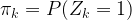


 is as above and
 . As we already have k, this amounts to sampling from the Gaussian distribution
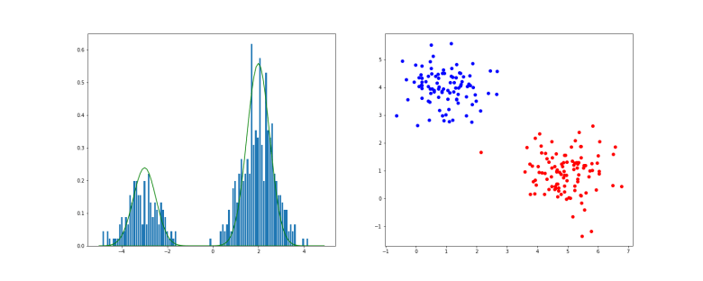


 . This series converges, and its value is

 for n, we obtain
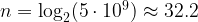
 .
.


 for a single point in the state space intractable.

 .
. 

 . We now calculate
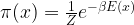
  according to the formula above. We then accept the proposal with probability
  . If the proposal is accepted, we set xn+1 = y, otherwise we set xn+1 = xn, i.e. we stay where we are.

 with probability one. This is very similar to a random search for a global maximum – we start at some point x, choose a candidate for a point with higher value of
  with a non-zero probability. This allows the algorithm to escape a local maximum much better. Intuitively, the algorithm will still try to spend more time in regions with large values of
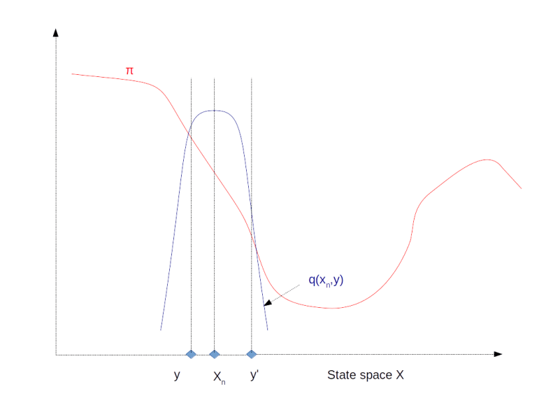
 and
and  ) approximated using the partial sums develops over time. We see that even though we still have huge spikes, the integral remains comparatively stable and converges already after a few thousand iterations. Even if we run the simulation only for 1000 steps, we already get close to the actual values zero (for
  (for
(for 
 and
and  are the standard deviations of X and Y. In our case, given a lag, i.e. a number l less than the length of the chain, we can form two samples, one consisting of the points
  and the second one consisting of the points of the shifted series
  . The autocorrelation with lag l is then defined to be the correlation coefficient between these two series. In the diagram, we can see how the autocorrelation depends on the lag. We see that for a large lag, the autocorrelation becomes small, supporting our intuition that the series and the shifted series become independent. However, if we execute several simulation runs, we will also find that in some cases, the convergence of the autocorrelation is very slow, so care needs to be taken when trying to obtain a nearly independent sample from the chain.
  , we can use the conditional probability given either x1 or x2 as a proposal distribution. Thus, we first fix x2, and draw a new value for x1 from the conditional probability for x1 given the current value of x2. Then we move to this new coordinate, fix x1, draw from the conditional distribution of x2 given x1 and set the new value of x2 accordingly. It can be shown (see for example