Learning algorithms for restricted Boltzmann machines – contrastive divergence

In the previous post on RBMs, we have derived the following gradient descent update rule for the weights.

In this post, we will see how this update rule can be efficiently implemented. The first thing that we note is that the term that appears several times is simply the conditional probability for the hidden unit j to be “on” and, as only the values 0 and 1 are possible, at the same time the conditional expectation value of that unit given the values of the visible units – let us denote this quantity by . Our update rule now reads

Theoretically, we know how to calculate this. The first term – the positive phase – is easy, this is just the average over the sample set.

The second term is more challenging. Theoretically, we would need a Gibbs sampler to calculate it using a Monte Carlo approach. One step of this sampler would proceed as follows.

1. Given the values v of the visible units, calculate the resulting expectation values e
2. Set hidden unit j to one with probability e_j
3. For each visible unit i, calculate the conditional probability p_i to be one given the new values of the hidden units
4. Set v_i to 1 with probability p_i

After some burn-in phase, we would then calculate the product after each step and take the average of these values.

The crucial point is that for a naive implementation, we would start the Gibbs sampling procedure during each gradient descent iteration from scratch, i.e. with some randomly initialized values for the visible units. One of the ideas behind the algorithm known as contrastive divergence that was proposed by G. Hinton in [1] is to restart the Gibbs sampler not at a random value, but a randomly chosen vector from the data set! The idea behind this is that if we have been running the training for some time, the model distribution should be close to the empirical distribution of the data, so sampling a vector from the data should give us something close to the equilibrium state of the Gibbs sampling Markov chain (if you do not known what a Markov chain is – do not worry and just read on, I will cover Markov chains and the mathematics behind all this in a later post).

The second approximation that the contrastive divergence algorithm makes is to replace the expectation values in the positive and negative phase by a point estimate. For the positive phase, that means we simply calculate the value at one point from the data set. For the negative phase, we run the Gibbs sampling procedure – starting as explained above with a vector from the data set – and then simply compute the product for the result.

It now turns out that, based on empirical observations, these approximations work extremely well – in fact, it turns out that instead of running a full Gibbs sampler with a few hundred or even a few thousand steps, one step is often sufficient! This is surprising, but open to an intuitive explanation – we run all this within the outer loop provided by the gradient descent algorithm, and if we chose the learning rate sufficiently small, the parameters do not change a lot between these steps, so that we effectively do something that is close to one long Gibbs sampling Markov chain.

With these simplifications, the constrastive divergence algorithm now looks as follows.

FOR EACH iteration DO

Sample a vector v from the data set

SET

FOR EACH hidden unit DO

SET with probability

FOR EACH visible unit DO

SET with probability

SET

SET

SET

SET

DONE

The first six lines within an iteration constitute one Gibbs sampling step, starting with a value for the visible units from the data set, sampling the hidden units from the visible units and sampling the visible units from the hidden units. In the next line, we recalculate the expectation values of the hidden units given the (updated) values of the visible units. The value is then the contribution of the negative phase to the update of . We can summarize the contributions for all pairs of indices as the matrix . Similarly, the positive phase contributes with . In the next line, we update W with both contributions, where is the learning rate. We then apply similar update rules to the bias for visible and hidden units – the derivation of these update rules from the expression for the likelihood function is done similar to the derivation of the update rules for the weights as shown in my last post.

Let us now implement this in Python. To have a small data set for our tests, we will use an artificial data set called bars and stripes that I have seen first in [3]. Given a number N, we can create an image with N x N pixels for every number x smallers than 2^N as follows. Each row corresponds to one binary digit of x. If this digit is one, the entire row is black, i.e. we have one black vertical stripe, otherwise the entire row is white. A second row of patterns is obtained by coloring the columns similarly instead of the rows. Thus we obtain 2^N+1 possible patterns, more than enough for our purposes. I have written a helper class BAS in Python that creates these patterns.

Next, let us turn to the actual RBM. We store the current state of the RBM in a class RBM that is initialized as follows.

class RBM:

    def __init__ (self, visible = 8, hidden = 3, beta = 1):
        self.visible = visible
        self.hidden = hidden
        self.beta = beta
        self.W = np.random.normal(loc = 0, scale = 0.01, size = (visible, hidden))
        self.b = np.zeros(shape = (1,visible))
        self.c = np.zeros(shape = (1,hidden))

Here W is the weight matrix, beta is the inverse temperature, and b and c are the bias vectors for the visible and hidden units.

Next we need a method that runs one step in a Gibbs sampling chain, starting with a state of the visible units captured in a matrix V (we calculate this in a mini-batch for more than one sample at a time, each row in the matrix represents one sample vector). Using once more the numpy library, this can be done as follows.

def runGibbsStep(self, V, size = 1):
    #
    # Sample hidden units from visible units
    #
    E = expit(self.beta*(np.matmul(V, self.W) + self.c))
    U = np.random.random_sample(size=(size, self.hidden))
    H = (U <= E).astype(int)
    #
    # and now sample visible units from hidden units
    #
    P = expit(self.beta*(np.matmul(H, np.transpose(self.W)) + self.b))
    U = np.random.random_sample(size=(size, self.visible))
    return (U <= P).astype(int), E

With this method at hand – which returns the new value for the visible units but the old value for the conditional expectation of the hidden units – we can now code our training routine.

def train(self,  V, iterations = 100, step = 0.01):
    batch_size = V.shape[0]
    #
    # Do the actual training. First we calculate the expectation
    # values of the hidden units given the visible units. The result
    # will be a matrix of shape (batch_size, hidden)
    #
    for _ in range(iterations):
        #
        # Run one Gibbs sampling step and obtain new values
        # for visible units and previous expectation values
        #
        Vb, E = self.runGibbsStep(V, batch_size)
        #
        # Calculate new expectation values
        #
        Eb = expit(self.beta*(np.matmul(Vb, self.W) + self.c))
        #
        # Calculate contributions of positive and negative phase
        # and update weights and bias
        #
        pos = np.tensordot(V, E, axes=((0),(0)))
        neg = np.tensordot(Vb, Eb, axes=((0),(0)))
        dW = step*self.beta*(pos -neg) / float(batch_size)
        self.W += dW
        self.b += step*self.beta*np.sum(V - Vb, 0) / float(batch_size)
        self.c += step*self.beta*np.sum(E - Eb, 0) / float(batch_size)

Let us now play around with this network a bit and visualize the training results. To do this, clone my repository and then run the simulation using

$ git clone  https://github.com/christianb93/MachineLearning.git
$ cd MachineLearning
$ python RBM.py  --run_reconstructions=1 --show_metrics=1

This will train a restricted Boltzmann machine on 20 images out of the BAS dataset with N=6. For the training, I have used standard parameters (which you can change using the various command line switches, use --help to see which parameters are available). The learning rate was set to 0.05. The number of iterations during training was set to 30.000, and 16 hidden units are used. The inverse temperature is set to 2.0. In each iteration, a mini-batch of 10 patterns is trained.

After every 500 iterations, the script prints out the current value of the reconstruction error. This is defined to be the norm of the difference between the value of the visible units when the Gibbs sampling step starts and the value after completing the Gibbs sampling step, i.e. this quantity measures how well the network is able to reconstruct the value of the visible units from the hidden units alone.

After the training phase is completed, the script will select eight patterns randomly. For each of these patterns, it will flip a few bits and then run 100 Gibbs sampling steps. If the training was successful, we expect that the result will be a reconstruction of the original image, i.e. the network would be able to match the distorted images to the original patterns.

When all the calculations have been completed, the network will display two images. The first image should roughly look like the image below.

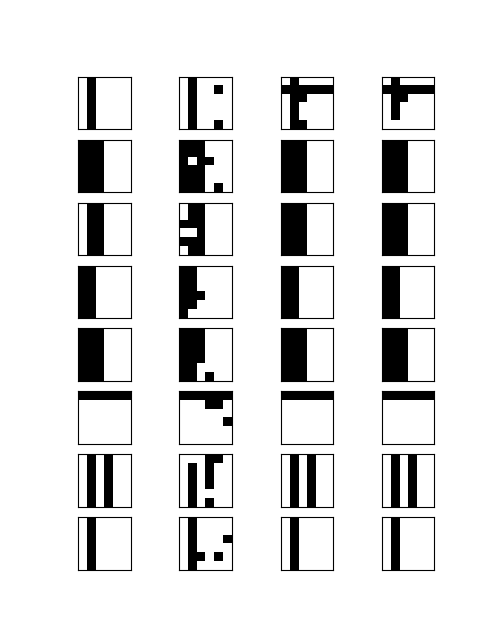
This matrix visualizes the result of the reconstruction process described above. Each of the rows shows the outcome for one of the eight selected patterns. The first image in each row is the original pattern from the BAS data set. The second one is the distorted image some pixels have been flipped. The third image shows the result of the reconstruction run after 50 Gibbs iterations, and the last image shows the result after the full 100 iterations.

We see that in most cases, the network is able to correctly reconstruct the original image. However, there are also a fes rows that look suspicious. In the first row, we could hope that the network eventually converges if we execute more sampling steps. In the third row, however, the network converges to a member of the BAS data set, but to the wrong one.

The second diagram that the script produces displays the change to the weights after each iteration and the reconstruction error.

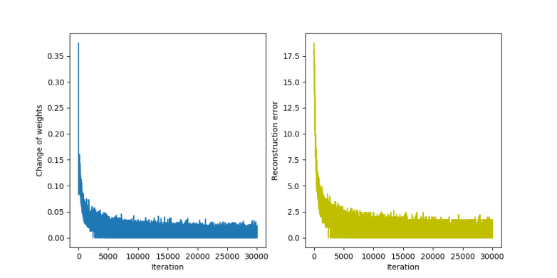
We see that both quantities quickly get smaller, but never stabilize at exactly zero. This is not really surprising – as we work with a non-zero temperature, we will always have some thermal fluctuations and the reconstruction error will never be constantly zero, but oscillate around a small value.

I invite you to play around with the parameters a bit to see how the network behaves. We can change the value of the inverse temperature with the parameter --beta, the number of hidden units with the parameter --hidden, the number of Gibbs steps used during the reconstruction with --sample and the step size with --step. If, for instance, you raise the temperature, the fluctuations of the reconstruction error will increase. If, one the other hand, we choose a very small temperature, the network converges very slowly. Making the step size too small or too large can also lead to non-convergence etc.

That completes this post on contrastive divergence. In the next post, I will show you an alternative algorithm that has gained a lot of popularity called persistent contrastive divergence (PCD), before we finally set out to implement an restricted Boltzmann machine on a GPU using the TensorFlow framework.

1. G. Hinton, Training products of experts by minimizing contrastive divergence, Journal Neural Computation Vol. 14, No. 8 (2002), 1771 1800
2. G. Hinton, A practical guide to training restricted Boltzmann machines, Technical Report University of Montreal TR-2010-003 (2010)
[3] D. MacKay, Information Theory, Inference and learning
algorithms, section 43, available online at this URL