Hopfield networks: theory

Having looked in some detail at the Ising model, we are now well equipped to tackle a class of neuronal networks that has been studied by several authors in the sixties, seventies and early eighties of the last century, but has become popular by an article [1] published by J. Hopfield in 1982.

The idea behind this and earlier research is as follows. Motivated by the analogy between a unit in a neuronal network and a neuron in a human brain, researchers were trying to understand how the neurons needed to be organized to be able to create abilities like associative memories, i.e. a memory that can be navigated by associations that bring up additional stored memories. To explain how the human brain organizes the connections between the neurons in optimal (well, as least useful) way, analogies with physical systems like the Ising model covered in this post which also exhibit some sort of spontaneous self organization, were pursued.

In particular, the analogy with stability attracted attention. In many physical systems, there are stable states. If the system is put into a state which is sufficiently close to such a stable state, it will, over time, move back into that stable state. A similar property is desirable for associative memory systems. If, for instance, such a system has memorized an image and is then placed in a state which is somehow close to that image, i.e. only a part of the image or a noisy version of the image is presented, it should converge into the memorized state representing the original image.

With that motivation, Hopfield described the following model of a neuronal network. Our network consists of individual units that can be in any of two states, “firing” and “not firing”. The system consists of N such units, we will denote the state of unit i by $s_i$ .

Any two units can be connected, and there is a matrix W whose elements represent the strength of the connection between the individual units, i.e. $w_{ij}$ is the strength of the connection between the units i and j. We assume that no neuron is connected to ifself, i.e. that $w_{ii} = 0$ , and that the matrix of weights is symmetric, i.e. that $w_{ij} = w_{ji}$ .

The activation of unit i is then obtained by summing up the weighted values of all neurons connected to it, i.e. given by

$a_i = \sum_j w_{ij} s_j$

Hopfield used a slightly different notation in his paper and assigned the values 0 and 1 to the two states, but we will again use -1 and +1.

So how does the Hopfield network operate? Suppose that the network is in a certain state. i.e. some of the neurons will be “firing”, represented by the value +1, and others will be passive, represented by the value -1. We now choose a neuron at random and calculate its activation function according to the formula above. We then determine the new state by the rule

$s_i' = \begin{cases} +1 & a_i \geq 0 \\ -1 & a_i < 0 \end{cases}$

In most cases, the network will actually converge after a finite number of steps, i.e. this rule does not change the state any more. To see why this happens, let us consider the function

$E(s) = - \frac{1}{2} \sum_{i,j} w_{ij} s_i s_j$

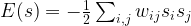
which is called the energy function of the model. Suppose that we pass from a state s to a state s’ by applying the update rule above. Let us assume that we have updated neuron i and changed its state from $s_i$ to $s_i'$ . Let

$\Delta s_i = s_i' - s_i$

Using the fact that the matrix W is symmetric, we can then write

$E(s') = -\frac{1}{2} \sum_{p,q \neq i} s_p s_q - \sum_p w_{pi} s_i' s_p$

which is the same as

$-\frac{1}{2} \sum_{p,q \neq i} s_p s_q - \sum_p w_{pi} s_i s_p - \sum_p w_{pi} (s_i' - s_i) s_p$

Thus we find that

$E(s') = E(s) - \Delta s_i \sum_p w_{ip} s_p$

Now the sum is simply the activation of neuron i. As our update rule guarantees that the product of $\Delta s_i$ and the activation of unit i is never negative, this implies that during the upgrade process, the energy function will always increase or stay the same. Thus the state will settle in a local minimum of the energy function.

At this point, we can already see some interesting analogies with the Ising model. Clearly, the units in a Hopfield network correspond to the particles in an Ising model. The state (firing or not) corresponds to the spin (upward or downward). The energy is almost literally the same as the energy of the Ising model without an external magnetic field.

Also the update rules are related. Recall that during a Gibbs sampling step for an Ising model, we calculate the conditional probability

$P = \sigma(2 \beta \langle J_i, s \rangle)$

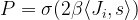
Here the scalar product is the equivalent of the activation, and we could rewrite this as

$P = \sigma(2 \beta a_i)$

Let us now assume that the temperature is very small, so that $\beta$ is close to infinity. If the activation of unit i is positive, the probability will be very close to one. The Gibbs sampling rule will then almost certainly set the spin to +1. If the activation is negative, the probability will be zero, and we will set the spin to -1. Thus the update role of a Hopfield network corresponds to the Gibbs sampling step for an Ising model at temperature zero.

At nonzero temperatures, a Hopfield network and an Ising model start to behave differently. The Boltzmann distribution guarantees that the state with the lowest energies are most likely, but as the sampling process proceeds, the random element built into the Gibbs sampling rule implies that a state can evolve into another of higher energy as well, even though this is unlikely. For the Hopfield network, the update rule is completely deterministic, and the states will always evolve into states of lower or at least equal energy.

The memories that we are looking for are now the states of minimum energy. If we place the system in a nearby state and let it evolve according to the update rules, it will move over time back into a minimum and thus “remember” the original state.

This is nice, but how do we train a Hopfield network? Given some state s, we want to construct a weight matrix such that s is a local minimum. More generally, if we have already defined weights giving some local minima, we want to adjust the weights in order to create an additional minimum at s, if possible without changing the already existing minima significantly.

In Hopfields paper, this is done with the following learning rule.

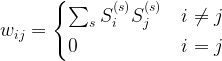
$w_{ij} = \begin{cases} \sum_s S^{(s)}_i S^{(s)}_j & i \neq j \\ 0 & i = j \end{cases}$

where $S^{(1)}, \dots, S^{(K)}$ are the states that the network should remember (in a later post in this series, we will see that this rule can be obtained as the low temperature limit of a training algorithm called contrastive divergence that is used to train a certain class of Boltzmann machines).

Thus a state S contributes with a positive value to $w_{ij}$ if $S_i$ and $S_j$ have the same sign, i.e. are in the same state. This corresponds to a rule known as Hebbian learning rule that has been postulated as a principle of learning by D. Hebb and basically states that during learning, connections between neurons are enforced if these neurons fire together ([2], chapter 4).

Let us summarize what we have done so far. We have described a Hopfield network as a fully connected binary neuronal network with symmetric weight matrices and have defined the update rule and the learning rule for these networks. We have seen that the dynamics of the network resembles that of an Ising model at low temperatures. We now expect that a randomly chosen initial state will converge to one of the memorized states and that therefore, this model can serve as an associative memory.

In the next post, we will put this to work and implement and train a Hopfield network in Python to study its actual behavior.

References

1. J. Hopfield, Neural networks and physical systems with emergent collective computational abilities, Proc. Nat. Acad. Sci. Vol. 79, No. 8 (1982), pp. 2554-2558
2. D.O. Hebb, The organization of behaviour, Wiley, New York 1949

Hopfield networks: theory

References

Published by christianb93

2 Comments

Leave a Comment Cancel reply

References

Share this:

Like this:

Related

Published by christianb93

2 Comments

Leave a Comment Cancel reply