The Boltzmann distribution

Boltzmann machines essentially learn statistical distributions. During the training phase, we present them a data set called the sample data that follows some statistical distribution. As the weights of the model are adjusted as part of the learning algorithm, the statistical model represented by the Boltzmann machine changes, and the learning phase is successful if the model gets as closely to the training data as possible.

The distribution that is learned by a Boltzmann machine is called a Boltzmann distribution (obviously, this is where the name comes from…) and is of great importance in statistical physics. In this post, we will try to understand how this distribution arises naturally from a few basic assumptions in statistical mechanics.

The first thing that we will need is a state space. Essentially, a state space is a (probability) space whose points are in one-to-one correspondence with the physical states of the system that we want to describe. To illustrate this, suppose you are given a system of identical particles. These particles can move freely in a certain are of space. The location of each individual particle can be described by its location in space, thus by three real numbers, and its velocity is described by three additional real numbers, one for each spatial component of the velocity. Thus as a state space for a single particle, we could choose a six-dimensional euclidian space. For a system of N particles, we would therefore need a state space of dimension 6N.

But a state space does not need to be somehow related to a position in some physical space. As another example, consider a solid, modeled as N particles with fixed locations in space. Let us also assume that each of these particles has a spin, and that this spin can either point upwards or downwards. We could then describe the spin of an individual particle by +1 (spin up) or -1 (spin down), and therefore our state space for N particles would be

$\Omega = \{-1, +1\}^N$

For every point s in the state space, i.e. for every possible state of the system, we assume that we can define an energy E(s), so that the energy defines a function E on the state space. One of the fundamental questions of statistical physics is now:

Given a state space and an energy function E on that space, derive, for each state s, the probability that the system is in the state s

What exactly do we mean by the probability to be in a specific state? We assume that we could theoretically construct a very large number of identical systems that are isolated against each other and independent. All these systems evolve according to the same rules. At any point in time, we can then pick a certain state and determine the fraction of systems that are in this state. This number is the probability to be in that state. The set of all these systems is called a statistical ensemble. The assignment of a probability to each state then defines a probability distribution on the state space. To avoid some technicalities, we will restrict ourselves to the case that the state space is finite, but of course more general cases can be considered as well.

As it stands, the question phrased above is impossible to answer – we need some additional assumptions on the system to be able to write down the probability distribution. We could, for instance, assume that the number of particles and the energy are fixed. A bit less restrictive is the assumption that the energy can vary, but that the temperature of the system (and the number of particles as well as the volume) is fixed – this is then called a canonical ensemble. Let us denote the temperate by T and assume now that it is constant.

We could describe a system for which these assumptions hold as being in contact with a second, very large system which is able to supply (or absorb) a virtually infinite amount of heat – this system is called a heat bath or thermal reservoir. The composite system that consists of our system of interest and the heat bath is assumed to be fully isolated. Thus its energy and the number of particles is constant. Our primary system can exchange heat with the heat bath and therefore its energy can change, while its temperate will stay constant and equal to the temperature of the heat bath.

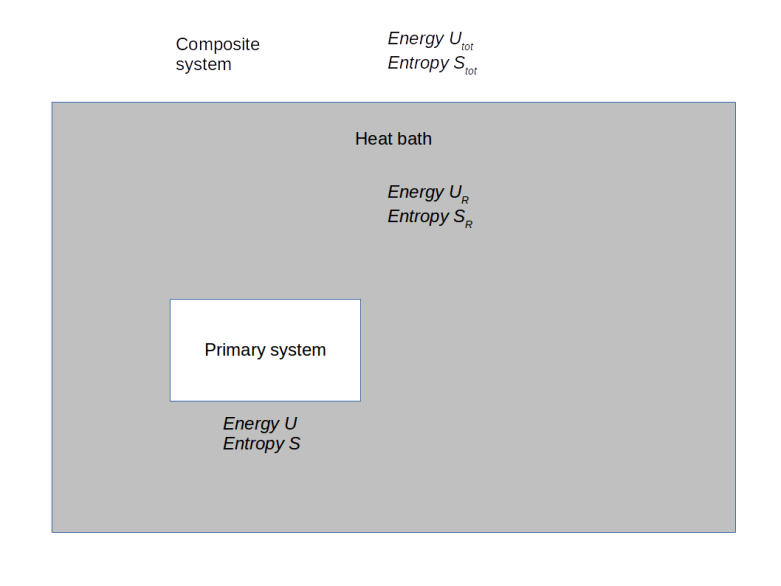
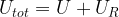
Let us denote the energy of the overall system by $U_{tot}$ , its entropy by $S_{tot}$ , the energy of the heat bath by $U_R$ and the entropy of the heat bath by $S_R$ (if energy and entropy are new concepts for you, I recommend my short introduction to thermodynamics which summarizes the most important fundamentals of thermodynamics on roughly 40 pages and also contains more details on statistical ensembles and the Boltzmann distribution).

Now it turns out that making only these very general assumptions (in contact with heat bath, constant temperature) plus one additional assumption, we can already derive a formula for the probability distribution on the state space – even without knowing anything else on the state space! Let me sketch the argument to get a feeling for it, more details can be found in the document mentioned above.

Let us assume that we are given some state s of our primary system with energy E(s). We can combine this state with a state of the heat bath to an allowed state of the composite system if the energies of both states add up to the total energy $U_{tot}$ , i.e. with any state of the heat bath which has energy $U_{tot} - E$ . Let us denote the number of states of the heat bath with that energy by

$W_R(U_{tot} - E)$

and let $W_{tot}$ denote the number of states of the composite system with energy $U_{tot}$ . The major additional assumption that we now make is that for the composite system, all states with energy $U_{tot}$ are equally likely – this is known as the principle of indifference.

Let us take a moment to reflect on this. The principle of indifference (sometimes called the principle of insufficient reason) states (translated into our case) that if the states of the system cannot be distinguished by any of the available observable quantities (in this case the energy which is equal to $U_{tot}$ for all states of the composite system), all these states should be assigned equal probabilities. This appears somehow reasonable, if one state was more likely than any other state, this state would somehow be distinguished but could not be told apart by any of the measurable quantities. Of course, that something is not measurable does not mean that it does not exist – there could even be a quantity that is theoretically observable and distinguishes certain states, but is simply not on our radar. So this principle has to be applied with care, but it turns out that the resulting distribution gives a surprisingly good description of what we can measure in a large number of applications, so this assumption is somehow justified by its success (see also {1] chapter 15 and 21 for a short discussion and justification).

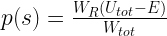
What does the principle of indifference imply for our primary system? The number of states of the composite system for which our primary system is in state s is exactly $W_R(U_{tot} - E)$ , because every such state combines with s to an admissible state of the composite system. If all these states are equally likely, the probability for s is therefore just the fraction of these states among all possible states of the composite system, i.e.

$p(s) = \frac{W_R(U_{tot} - E)}{W_{tot}}$

The beauty of this equation is that we can express both, the numerator and the denominator, by the entropy. And this is where finally the Austrian physicist Ludwig Boltzmann comes into play. Boltzmann identified the entropy of a system with the logarithm of the number of states available to the system – that is the famous relation that is expressed as

$S = k \ln W$

on his tomb stone. Here W is the number of states available to the system, and k is the Boltzmann constant.

Let us now use this expression for both numerator and denominator. We start with the denominator. If the system has reached thermal equilibrium, the primary system will have a certain energy U which is related to the total energy and the energy of the reservoir by

$U_{tot} = U + U_R$

Using the additivity of the entropy, we can therefore write

$W_{tot} = \exp \frac{1}{k} \left[ S(U) + S_R(U_{tot} - U) \right]$

Observe that we assume the number of particles and the volume of both the reservoir and the composite system to be constant, so that the entropy does really only depend on the volume (or at least we assume that the dependency on the volume is negligible). For the numerator, we need a different approach. Let us try a Taylor expansion around the energy 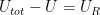$U_{tot} - U = U_R$ . The first derivative of the entropy with respect to the energy is – by definition – the inverse of the temperature:

$\frac{\partial S_R}{\partial U_R} = \frac{1}{T}$

The second derivative turns out to be related to the heat capacity $C_R$ of the reservoir. In fact, we have

$\frac{\partial}{\partial U_R} \frac{1}{T} = - \frac{1}{T^2 C_R}$

Now a heat bath is characterised by the property that we can add a virtually infinite amount of heat without raising the temperature. Thus the heat capacity is infinite, and the second derivative is (virtually) zero. Therefore our Taylor expansion is

$S_R(U_{tot} - E(s)) = S_R(U_{tot} - U) + \frac{1}{T} (U - E(s))$

Putting all this together, a few terms cancel out, and we find that

$p(s) = \exp \frac{1}{kT} \left[ (U - TS(U)) - E(s) \right]$

Now the energy U is the average, i.e. the macroscopically observable, energy of the primary system. Therefore $U - TS$ is the Helmholtz energy $F$ . If we also introduce the usual notation $\beta$ for the inverse of $kT$ , we finally find that

$p(s) = e^{\beta F} e^{- \beta E(s)}$

This is usually written down a bit differently. To obtain this form, let us sum this over all possible states. As U and therefore F are averages and do not depend on the actual state, but all probabilities have to add up to one, we find that

$1 = e^{\beta F} \sum_s e^{- \beta E(s)}$

The last sum is called the partition function and usually denoted by Z. Therefore we obtain

$p(s) = \frac{1}{Z} e^{- \beta E(s)}$

which is the Boltzmann distribution as it usually appears in textbooks. So we have found a structurally simple expression for the probability distribution, starting with a rather general set of assumptions.

Note that this equation tells us that the state with the lowest energy will have the highest probability. Thus the system will prefer states with low energies, and – due to the exponential – states with a significantly higher energy tend to be very unlikely.

Due to the very mild assumptions, the Boltzmann distribution applies to a large range of problems – it can be used to derive the laws for an ideal gas, for systems of spins in a solid or for a black body. However, the formula is only simple at the first glance – the real complexity is hidden in the partition function. With a few short calculations, one can for instance show that the entropy can be derived from the partition function as

$S = k \frac{\partial}{\partial T} T \ln Z$

Thus if we known the partition function as a function of the macroscopic variables, we know all the classical thermodynamical quantities like entropy, temperature and Helmholtz energy. In many cases, however, the partition function is not known, and we have to devise techniques to derive physically interesting results without a tractable expression for the partition function.

That was it for today. This blog was a bit theoretical, so next time we will apply this to a concrete model which is accessible for numerical simulations, namely the Ising model. Until then, you might want to go through my notes which contain some details on the Boltzmann distribution as well as examples and applications.

References

1. H.B. Callen, Thermodynamics and an introduction to thermostatistics, 2nd edition, John Wiley 1985
2. D.V. Schroeder, An introduction to thermal physics, Addison Wesley 2000

The Boltzmann distribution

References

Published by christianb93

4 Comments

Leave a Comment Cancel reply

References

Share this:

Like this:

Related

Published by christianb93

4 Comments

Leave a Comment Cancel reply