Python – LeftAsExercise

The nuts and bolts of VertexAI – managed datasets

Ultimately, VertexAI is about the processing of data. In previous posts in this series, we have placed our data in a GCS bucket and referenced it within our pipelines directly by the URI – you could call this a self-managed dataset. Alternatively, VertexAI also allows you to defined managed datasets which are stored in a central registry, a feature which we will explore today.

Tabular datasets

The first thing that you have to understand when working with VertexAI datasets is that they come in different flavours called types and objectives in the VertexAI console. The type is more than an attribute, and we will see that for instance tabular datasets which we will look at first behave fundamentally different from other types of datasets like text datasets.

To get started, let us create a small tabular dataset with sample data. I have added a simple script to my repository for this series that will build a small dataset in CSV format with two columns, populated with random data. Run the script

python3 datasets/create_csv.py

and upload the resulting file data.csv to the GCS bucket that you should have created as part of the initial setup for this series.

gsutil cp \
  data.csv \
  gs://vertex-ai-$GOOGLE_PROJECT_ID/datasets/my-dataset.csv

Now we can import this dataset into the VertexAI data registry. For that purpose, open the Google cloud console and use the navigation bar at the left to visit “Vertex AI – Datasets”. Make sure to select the region that you are using and click on “Create dataset”. You should see a screen similar to the one below.

Enter “my-dataset” as dataset name at the top, then select “Tabular” and “Regression / classification”. Click on “Create”.

You will now be taken to a screen that gives you different options to actually import data into your newly created dataset. Select the CVS file that we have just uploaded to GCS as a GCS source.

If you now hit “Continue”, Google will link the URI of your CSV file to the dataset. Note that in that sense, a tabular dataset is more or less a reference to a physical dataset located somewhere in a GCS bucket. Vertex AI does not create a copy, so if you modify the CSV file, this will modify the dataset.

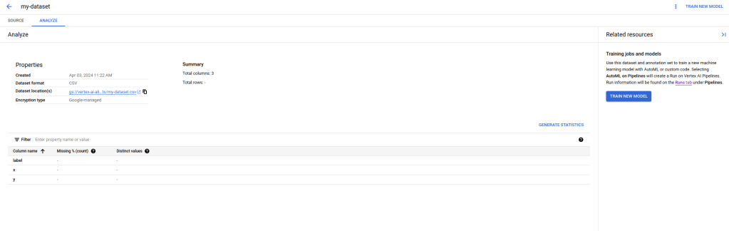
You now have several options to proceed. You can follow the link displayed on the right hand side to use Vertex AIs AutoML feature which will train a regression model on your data from scratch (be careful, there is an extra charge associated with that which goes far beyond the cost for the actual compute capacity needed, so do not do this if you just want to play). You can also analyze the data by clicking on the link “Generate statistics”.

Be patient, even for our tiny sample with 2000 items, this will take some time – when I tried this, it took about ten minutes. As a result, you will get the count of distinct values per column, and Vertex AI would also inform you about any missing values.

Let us now try to collect a bit more information on our dataset by using the Python API. The high-level API defines APIs which are specific for a given dataset type, but there is also an API that we can use to get information for an arbitrary dataset. Our repository contains an example that demonstrates how to use this in datasets/get_dataset.py. Let us run this.

python3 datasets/get_dataset.py

If you look at the output, you will find that it references a metadata schema that is in fact specific to the type of dataset that we have defined. The metadata schema is the URI of a file on GCS, and you can of course use gsutil to download a copy of this.

gsutil cp gs://google-cloud-aiplatform/schema/dataset/metadata/tabular_1.0.0.yaml .
more tabular_1.0.0.yaml

From this description, you will learn that a tabular dataset is really only a pointer to the data that is contains, which can either be stored in one or more files on GCS or in a BigQuery table. In addition to this, Google will only store some metadata like the creation time and a unique ID. Google will, however, add a metadata item to the metadata store that also references the dataset.

Text datasets

Let us now turn to a slightly more interesting type of datasets – text datasets. The basic workflow for text datasets is the same as for tabular datasets – we create the dataset (either via the SDK or on the console) and upload data. However, the format of the data is different – data is usually imported in JSON format that follows a specific schema which depends on the classification task. Let us use sentiment analysis as an example for which the schema is available here. Essentially, each item in our data (called a document) would be represented by a JSON object that looks as follows.

{
    "textContent" : "the actual text",
    "sentimentAnnotation": {
            "sentiment": 1,
            "sentimentMax": 2
    },
}

Here, the textContent is the actual data. The content of sentimentAnnotation – if present – contains the label, which consists of a score between 0 and maximal 10, and the sentimentMax value that specifies the maximum value (and should be the same for all documents in the set).

Instead of including the text content directly, the field textContent can also be replaced by a field textGcsUri which is the URI of a file stored on GCS, so that every record is represented by one file. Also note that only each line is valid JSON, while the full document is not – this is why the format is called JSON lines and has extension *.jsonl.

To try this, we again need a small sample dataset. As this is a series on Vertex AI, I could not resist the temptation to write a small script which asks Googles Gemini Pro model to do this for us. It uses few-shot learning to get a batch of ten records from the LLM, validates the content to see that it is valid, and repeats this until we have collected 100 valid documents which are then written to a file text.jsonl. You can either run this yourself

python3 datasets/generate_text_data.py

or use the file that I have included in the repository

cp datasets/text.jsonl .

In any case, we will again have to copy the file that you want to use to a GCS bucket as we did it before for the tabular dataset.

gsutil cp \
  text.jsonl \
  gs://vertex-ai-$GOOGLE_PROJECT_ID/datasets/text.jsonl

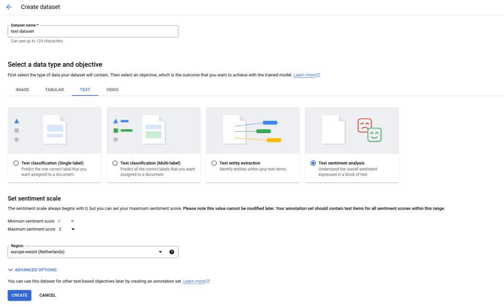
Once the upload is complete, you can create a dataset using the same workflow as for our tabular dataset, with the difference that you will have to select a text dataset with the objective sentiment analysis. Also note that you will have to specify the minimum and maximum sentiment score (0 and 2 in our case) and you will have to use a location that supports this feature which is not yet available in all locations. Let us call our dataset “text-dataset”.

Then proceed with the import as before by selecting the GCS location of the text.jsonl file that we have uploaded earlier. Again, the import takes some time. Note that the test data set that is included in the repository does actually contain duplicates, so when the import completes, you will only see 98 records, not 100 – this nicely demonstrates that Google does some work behind the scenes while you are waiting.

Let us now take a closer look at our dataset by running the script again that we have already used to display our tabular dataset, specifying the name and region of our new dataset – be sure to use the same region here as the one that you have selected when creating the dataset.

python3 datasets/get_dataset.py \
  --dataset=text-dataset \
  --region=europe-west4

If you compare this to the output for our tabular dataset, you should see two interesting differences. First, this dataset has a different schema reflecting the fact that this is a text dataset, not a tabular dataset. Second the GCS bucket that is displayed is not the bucket that we have used for the upload, but a bucket that Google has generated for us. This reflects the fact that this time, the data itself is managed by Google and is more than just a reference.

It is instructive to actually visit the GCS bucket that Google has generated (which will be owned by you, so you can actually see it). You will find that behind the scenes, Google has created one blob for every item in the input. This allows the platform to also modify each item separately, and in fact, in the console window for this dataset, you can edit individual items and add, remove or change labels.

Corresponding to this, you can also export your dataset, either directly from the console or programmatically using the export_data method of the DatasetServiceClient. Here, exporting means that the data will be written to a GCS location of your choice from where you can further process it – I would not recommend to directly use the bucket controlled by Google for this purpose as this is supposed to be managed by Google exclusively.

This closes our short series on Vertex AI. Of course, there are many features that we have not yet touched upon, like notebook and the workbench, batch predictions, feature stores or the new platform components with GenAI specific services like the model garden, LLMs and vector storage. However, with the basic understanding that you will have gained if you have followed me up to this point, you should be well prepared to explore these features as well.

Mastering large language models Part XV: building a chat-bot with DialoGPT and Streamlit

Arguably, a large part of the success of models like GPT is the fact that they have been equipped with a chat frontend and proved able to have a dialogue with a user which is perceived as comparable to a dialogue you would have with another human. Today, we will see how transformer based language models can be employed for that purpose.

In the previous post, we have seen how we can easily download and run pretrained transformer models from the Huggingface hub. If you play with my notebook on this a bit, you will soon find that they do exactly what we expect them to do – find the most likely completion. If, for instance, you use the promt “Hello”, followed by the end-of-sentence token tokenizer.eos_token, they will give you a piece of text starting with “Hello”. This could be, for instance, a question that someone has posted into a Stackexchange forum.

If you want to use a large language model to build a bot that can actually have a conversation, this is usually not what you want. Instead, you want a completion that is a reply to the prompt. There are different ways to achieve this. One obvious approach that has been taken by Microsoft for their DialoGPT model is to already train the model (either from scratch or via fine-tuning) on a dataset of dialogues. In the case of DialoGPT, the dataset has been obtained by scraping from Reddit.

A text-based chat-bot

Before discussing how to use this model to implement a chat-bot, let us quickly fix a few terms. A conversation between a user and a chat-bot is structured in units called turns. A turn is a pair of a user prompt and a response from the bot. DialoGPT has been trained on a dataset of conversations, modelled as a sequence of turns. Each turn is a sequence of token, where the user prompt and the reply of the bot are separated by an end-of-sentence (EOS) token. Thus a typical (very short) dialogue with two turns could be represented as follows

Good morning!<eos>Hi<eos>How do you feel today?<eos>I feel great<eos>

Here the user first enters the prompt “Good morning!” to which the bot replies “Hi”. In the second turn, the user enters “How do you feel today” and the bot replies “I feel great”.

Now the architecture of DialoGPT is identical to that of GPT-2, so we can use what we have learned about this class of models (decoder-only models) to sample from it. However, we want the model to take the entire conversation that took place so far into account when creating a response, so we feed the entire history, represented as a sequence of token as above, into the model when creating a bot response. Assuming that we have a function generate that accepts a prompt and generates a reply until it reaches and end-of-sentence token, the pseudocode for a chat bot would therefore look as follows.

input_ids = []
while True:
    prompt = input("User:")
    input_ids.extend(tokenizer.decode(prompt))
    input_ids.append(tokenizer.eos_token)
    response = generate(input_ids)
    print(f"Bot: {tokenize.decode(response)}"
    input_ids.extend(response)

Building a terminal-based chat-bot on top of DialoGPT is now very easy. The only point that we need to keep in mind is that in practice, we will want to cache past keys and values as discussed in the last post. As we need the values again in the next turn which will again be based on the entire history, our generate function should return these values and we will have to pass them back to the function in the next turn. An implementation of generate along those lines can be found here in my repository. To run a simple text-based chatbot, simply do (you probably want to run this in a virtual Python environment):

git clone https://github.com/christianb93/MLLM
cd MLLM
pip3 install -r requirements.txt
cd chatbot
python3 chat_terminal.py

The first time you run this, the DialoGPT model will be downloaded from the hub, so this might take a few minutes. To select a different model, you can use the switch --model (use --show_models to see a list of valid values).

Using Streamlit to build a web-based chat-bot

Let us now try to build the same thing with a web-based interface. To do this, we will use Streamlit, which is a platform designed to easily create data-centered web applications in Python.

The idea behind Streamlit is rather simple. When building a web-based applicaton with Streamlit, you put together an ordinary Python script. This script contains calls into the Streamlit library that you use to define widgets. When you run the Streamlit server, it will load the Python script, execute it and render an HTML page accordingly. To see this in action, create a file called test.py in your working directory containing the following code.

import streamlit as st 


value = st.slider(label = "Entropy coefficient", 
          min_value = 0.0, 
          max_value = 1.0)
print(f"Slider value: {value}")

Then install streamlit and run the applications using

pip3 install streamlit==1.23.1 
streamlit run test.py

Now a browser window should open that displays a slider, allowing you to select a parameter between 0 and 1.

In the terminal session in which you have started the Streamlit server, you should also see a line of output telling you that the value of the slider is zero. What has happened is that Streamlit has started an HTTP server listening on port 8501, processed our script, rendered the slider that we have requested, returned its current value and then entered an internal event loop outside of the script that we have provided.

If now change the position of the slider, you will see a second line printed to the terminal containing the new value of the slider. In fact, if a user interacts with any of the widgets on the screen, Streamlit will simply run the script once more, this time returning the updated value of the slider. So behind the scenes, the server is sitting in an event loop, and whenever an event occurs, it will not – like frontend frameworks a la React will do it – use callbacks to allow the application to update specific widgets, but instead run the entire script again. I recommend to have a short look at the section “Data flow” in the Streamlit documentation which explains this in a bit more detail.

This is straightforward and good enough for many use cases, but for a chat bot, this creates a few challenges. First, we will have to create our model at some point in the script. For larger models, loading the model from disk into memory will take some time. If we do this again every time a user interacts with the frontend, our app will be extremely sluggish.

To avoid this, Streamlit supports caching of function values by annotating a function with the decorator st.cache_resource. Streamlit will then check the arguments of the function against the cached values. If the arguments match a previous call, it will directly return a reference to the cached response without actually invoking the function. Note that here a reference is returned, meaning in our case that all sessions share the same model.

The next challenge that we have is that our application requires state, for instance the chat history or the cached past keys and values, which we have to preserve for the entire session. To maintain session-state, Streamlit offers a dictionary-like object st.session_state. When we run the script for the first time, we can initialize the chat history and other state components by simply adding a respective key to the session state.

st.session_state['input_ids'] = []

For subsequent script iterations, i.e. re-renderings of the screen, that are part of the same session, the Streamlit framework will then make sure that we can access the previously stored value. Internally, Streamlit is also using the session state to store the state of widgets, like the position of a slider or the context of a text input field. When creating such a widget, we can provide the extra parameter key which allows us to specify the key under which the widget state is stored in the session state.

A third feature of Streamlit that turns out to be useful is to use conventional callback functions associated with a widget. This makes it much easier to trigger specific actions when a specific widget changes state, for instance if the user submits a prompt, instead of re-running all actions in the script every time the screen needs to be rendered. We can, for instance, define a widget that will hold the next prompt and, if the user hits “Return” to submit the prompt, invoke the model within the callback. Inside the callback function, we can also update the history stored in the session state.

def process_prompt():
    #
    # Get widget state to access current prompt
    #
    prompt = st.session_state.prompt
    #
    # Update input_ids in session state
    #
    st.session_state.input_ids.extend(tokenizer.encode(prompt))
    st.session_state.input_ids.append(tokenizer.eos_token_id)
    #
    # Invoke model
    #
    generated, past_key_values, _ = utils.generate(model = model, 
                                            tokenizer = tokenizer, 
                                            input_ids = st.session_state.input_ids, 
                                            past_key_values = st.session_state.past_key_values, 
                                            temperature = st.session_state.temperature, debug = False)
    response = tokenizer.decode(generated).replace('<|endoftext|>', '')
    #
    # Prepare next turn
    #
    st.session_state.input_ids.extend(generated)

Armed with this understanding of Streamlit, it is not difficult to put together a simple web-based chatbot using DialoGPT. Here is a screenshot of the bot in action.

You can find the code behind this here. To run this, open a terminal and type (switching to a virtual Python environment if required):

git clone https://github.com/christianb93/MLLM
cd MLLM
pip3 install -r requirements.txt
cd chatbot
streamlit run chat.py

A word of caution: by default, this will expose port 8501 on which Streamlit is listening on the local network (not only on localhost) – it is probably possible to change this somewhere in the Streamlit configuration, but I have not tried this.

Also remember that the first execution will include the model download that happens in the background (if you have not used that model before) and might therefore take some time. Enjoy your chats!

Mastering large language models – Part XII: byte-pair encoding

On our way to actually coding and training a transformer-based model, there is one last challenge that we have to master – encoding our input by splitting it in a meaningful way into subwords. Today, we will learn how to do this using an algorithm known as byte-pair encoding (BPE).

Let us first quickly recall what the problem is that subword encoding tries to solve. To a large extent, the recent success of large language models is due to the tremendous amount of data used to train them. GPT-3, for instance, has been trained on roughly 500 mio tokens (which, as we will see soon, are not exactly words) [3]. But even much smaller datasets tend to contain a large number of unique words. The WikiText103 dataset [4] for instance contains a bit more than 100 mio. words, which represent a vocabulary of 267.735 unique words. With standard word-level encoding, this would become a dimension in the input and output layers of our neural network. It is not hard to imagine that with 500 mio. token as input, this number would even be much larger and we clearly have a problem.

The traditional way to control the growth of the vocabulary is to introduce a minimum frequency. In other words, we could only include token in the vocabulary that occur more than a given number of times – the minimum frequency – in the training data and tune this number to realize a cap on the vocabulary size. This, however, has the disadvantage that during training and later inference, we will face unknown words. Of course we can reserve a special token for these unknown words, but still a translator would have to know how to handle them.

Character-level encoding solves the problem of unknown words, but introduces a new problem – the model first has to learn words before it can start to learn relations between words. In addition, if our model is capable of learning relations within a certain range L, it does of course make a difference whether the unit in which we measure this range is a character or a word.

This is the point where subword tokenization comes into play. Here, the general idea is to build up a vocabulary that consists of subword units, not full words – but also more than just individual characters. Of course, to make this efficient, we want to include those subwords in our vocabulary that occur often, and we want to include all individual characters. If we need to encode a word that consists of known subwords, we can use those, and in the worst case, we can still go down to the character level during encoding so that we will not face unknown words.

Byte-pair encoding that has first been applied to machine learning in [1] is one way to do this. Here, we build our vocabulary in two phases. In the first phase, we go through our corpus and include all characters that we find in our vocabulary. We then encode our data using this preliminary vocabulary.

In the second phase, we iterate through a process known as merge. During each merge, we go through our data and identify the pair of token in the vocabulary that occurs most frequently. We then include a new token in our vocabulary that is simply the concatenation of these two existing token and update our existing encoding. Thus every merge adds one more token to the vocabulary. We continue this process until the vocabulary has reached the desired size.

Note that in a real implementation, the process of counting token pairs to determine their frequency is usually done in two steps. First, we count how often an individual word occurs in the text and save this for later reference. Next, given a pair of token, we go through all words that contain this pair and then add up the frequencies of these words to determine the frequency of the token pair.

Let us look at an example to see how this works in practice. Suppose that the text we want to encode is

low, lower, newest, widest

In the first phase, we would build an initial vocabulary that consists of all characters that occur in this text. However, we want to make sure that we respect word boundaries, so we need to be able to distinguish between characters that appear within a word and those that appear at the end of the word. We do this by adding a special token </w> to a token that is located at the end of a word. In our case, this applies for instance to the character w that therefore gives rise to two entries in our vocabulary – w and w</w>. With this modification, our initial vocabulary is

'o', 'r</w>', 's', 'w</w>', 'n', 'i', 'e', 'l', 'd', 'w', 't</w>'

We now go through all possible combinations of two token and see how often the appear in the text. Here is what we would find in our example.

Token pair	Frequency
l + o	2
o + w</w>	1
o + w	1
w + e	2
e + r</w>	1
n + e	1
e + w	1
e + s	2
s + t</w>	2
w + i	1
i + d	1
d + e	1

We now pick the pair of token (usually called a byte-pair, even though this is strictly speaking of course not correct when we use Unicode points) that occurs most frequently. In our case, several byte pairs occur twice, and we pick one of them, say w and e. We now add an additional token “we” to our vocabulary and re-encode our text. With this vocabulary, our text which previously was represented by the sequence of token

l, o, w</w>, l, o, w, e, r</w>, n, e, w, e, s, t</w>, w, i, d, e, s, t</w>

would now be encoded as

l, o, w</w>, l, o, we, r</w>, n, e, we, s, t</w>, w, i, d, e, s, t</w>

Note the new token, marked with bold face, that appears at the two positions where we previously had the combination of the token w and e. This concludes our first merge.

We can now continue and conduct the next merge. Each merge will add one token to our vocabulary, so that controlling the number of merges allows us to create a vocabulary of the desired size. Note that each merge results in two outputs – an updated vocabulary and a rule. In our case, the first merge resulted in the rule w, e ==> we.

To encode a piece of text that was not part of our training data when running the merges, we now simply replay these rules, i.e. we start with our text, break it down into characters, corresponding to the token in the initial vocabulary, and apply the rules that we have derived during the merges in the order in which the merges took place. Thus to encode text, we need access to the vocabulary and to the rules.

Let us now turn to implementing this in Python. The original paper [1] does already contain a few code snippets that make an implementation based on them rather easy. As usual, this blog post comes with a notebook that, essentially based on the code in [1], guides you through a simple implementation using the example discussed above. Here are a few code snippets to illustrate the process.

The first step is to build a dictionary that contains the frequencies of individual words, which we will later use to easily calculate the frequency of a byte pair. Note that the keys in this dictionary are the words in the input text, but already broken down into a sequence of token, separated by spaces, so that we need to update them as we merge and add new token.

def get_word_frequencies(pre_tokenized_text):
    counter = collections.Counter(pre_tokenized_text)
    word_frequencies = {" ".join(word) + "</w>" : frequency for word, frequency in counter.items() if len(word) > 0}
    return word_frequencies

As the keys in the dictionary are already pretokenized, we can now build our initial vocabulary based on these keys.

def build_vocabulary(word_frequencies):
    vocab = set()
    for word in word_frequencies.keys():
        for c in word.split():
            vocab.add(c)
    return vocab

Next, we need to be able to identify the pair of bytes that occurs most frequently. Again, Python collections can be utilized to do this – we simply go through all words, split them into symbols, iterate through all pairs and increase the count for this pair that we store in a dictionary.

def get_stats(word_frequencies):
  pairs = collections.defaultdict(int)
  for word, freq in word_frequencies.items():
    symbols = word.split()
    for i in range(len(symbols)-1):
      pairs[symbols[i],symbols[i+1]] += freq
  return pairs

Finally, we need a function that executes an actual merge. During each merge, we use regular expressions (more on the exact expression that we use here can be found in my notebook) to replace each occurence of the pair by the new token.

def do_merge(best_pair, word_frequencies, vocab):
    new_frequencies = dict()
    new_token = "".join(best_pair)
    pattern = r"(?<!\S)" + re.escape(" ".join(best_pair)) + r"(?!\S)"
    vocab.add(new_token)
    for word, freq in word_frequencies.items():
        new_word = re.sub(pattern, new_token, word)
        new_frequencies[new_word] = word_frequencies[word]
    return new_frequencies, vocab

We can now combine the functions above to run a merge. Essentially, during a merge, we need to collect the statistics to identify the most frequent pair, call our merge function to update the dictionary containing the word frequencies and append the rule that we have found to a list of rules that we will save later.

stats = get_stats(word_frequencies)
best_pair = max(stats, key=lambda x: (stats[x], x)) 
print(f"Best pair: {best_pair}")
word_frequencies, vocab = do_merge(best_pair, word_frequencies, vocab)
rules.append(best_pair)

This code, howevers, is awfully slow, as it basically repeats the process of counting once with every merge. The authors of the original paper also provide a reference implementation [2] that applies some tricks like caching and the use of indices to speed up the process significantly. In my repository for this series, I have assembled an implementation that follows this reference implementation to a large extent, but simplifies a few steps (in particular the incremental updates of the frequency counts) and is therefore hopefully a bit easier to read. The code consists of the main file BPE.py and a test script test bpe.py.

The test script can also be used to compare the output of our implementation with the reference implementation [3]. Let us quickly do this using a short snippet from “War and peace” that I have added to my repository.

#
# Clone the reference implementation
#
git clone https://github.com/rsennrich/subword-nmt.git
cd subword-nmt
#
# Get files from my repository
#
wget https://raw.githubusercontent.com/christianb93/MLLM/main/bpe/BPE.py
wget https://raw.githubusercontent.com/christianb93/MLLM/main/bpe/test_bpe.py
wget https://raw.githubusercontent.com/christianb93/MLLM/main/bpe/test.in
wget https://raw.githubusercontent.com/christianb93/MLLM/main/bpe/test.rules
#
# Run unit tests
# 
python3 test_bpe.py
#
# Run reference implementation
#
cat test.in | python3 subword_nmt/learn_bpe.py -s=50 > rules.ref
#
# Run our implementation
#
python3 test_bpe.py --infile=test.in --outfile=rules.dat
#
# Diff outputs
#
diff rules.dat rules.ref
diff rules.ref test.rules

The only difference that the diff should show you is a header line (containing the version number) that the reference implementation adds which we do not include in our output, all the remaining parts of the output files which contain the actual rules should be identical. The second diff verifies the reference file that is part of the repository and is used for the unit tests.

Over time, several other subword tokenization methods have been developed. Two popular methods are Googles wordpiece model ([6], [7]) and the unigram tokenizer [8]. While wordpiece is very similar to BPE and mainly differs in the way how the next byte pair for merging is selected, the unigram tokenizer starts with a very large vocabulary, containing all characters and the most commonly found substrings, and then iteratively removes items from the vocabulary based on a statistic model.

With BPE, we now have a tokenization method at our disposal which will allow us to decouple vocabulary size from the size of the training data, so that we can train a model even on large datasets without having to increase the model size. In the next post, we will put everything together and train a transformer-based model on the WikiText dataset.

References:

[1] R. Sennrich et al., Neural Machine Translation of Rare Words with Subword Units
[2] https://github.com/rsennrich/subword-nmt
[3] T. Brown et al., Language Models are Few-Shot Learners
[4] https://blog.salesforceairesearch.com/the-wikitext-long-term-dependency-language-modeling-dataset/
[5] K. Bostrom, G. Durrett, Byte Pair Encoding is Suboptimal for Language Model Pretraining
[6] Y. Wu et al., Google’s Neural Machine Translation System: Bridging the Gap between Human and Machine Translation
[7] M. Schuster, K. Nakajima, Japanese and Korean voice search
[8] T. Kudo, Subword Regularization: Improving Neural Network Translation Models with Multiple Subword Candidates

Mastering large language models – Part IX: self-attention with PyTorch

In the previous post, we have discussed how attention can be applied to avoid bottlenecks in encoder-decoder architectures. In transformer-based models, attention appears in different flavours, the most important being what is called self-attention – the topic of todays post. Code included.

Before getting into coding, let us first describe the attention mechanism presented in the previous blog in a bit more general setting and, along the way, introduce some terminology. Suppose that a neural network has access to a set of vectors v_i that we call the values. The network is aiming to process the information contained in the v_i in a certain context and, for that purpose, needs to condense the information specific to that context into a single vector. Suppose further that each vector v_i is associated with a vector k_i called the key, that somehow captures which information the vector v_i contains. Finally assume that we are able to form a query vector q that specificies what information the network needs. The attention mechanism will then assemble a linear combination

$\textrm{attn}(q, \{k_i\}, \{v_i\}) = \sum_i \alpha(q, k_i) v_i$

called the attention vector.

To make this more tangible, let us look at an example. Suppose an encoder processes a sequence of words, represented by vectors x_i. While encoding a part of the sentence, i.e. a specific vector, the network might want to pull in some data from other parts of the sentence. Here, the query would be the currently processed word, while keys and values would come from other parts of the same sentence. As keys, queries and values all come from the same sequence, this form of attention is called self-attention. Suppose, for example, that we are looking at the sentence (once again taken from “War and peace”)

The prince answered nothing, but she looked at him significantly, awaiting a reply

When the model is encoding this sentence, it might help to pull in the representation of the word “prince” when encoding “him”, as here, “him” refers to “the prince”. So while processing the token for “him”, the network might put together an attention vector focusing mostly on the token for “him” itself, but also on the token for “prince”.

In this example, we would compute keys and values from the input sequence, and the query would be computed from the word we are currently encoding, i.e. “him”. A weight is then calculated for each combination of key and query, and these weights are used to form the attention vector, as indicated in the diagram above (we will see in a minute how exactly this works).

Of course, this only helps if the weights that we use in that linear combination are somehow helping the network to focus on those values that are most relevant for the given key. At the same time, we want the weights to be non-negative and to sum up to one (see this paper for a more in-depth discussion of these properties of the attention weights which are a bit less obvious). The usual approach to realize this is to first define a scoring function

$\textrm{score}(q, k_i)$

and then obtain the attention weights as a softmax function applied to these scores, i.e. as

$\alpha(q, k_i) = \frac{\exp(\textrm{score}(q, k_i))}{\sum_j \exp(\textrm{score}(q, k_j))}$

For the scoring function itself, there are several options (see Effective Approaches to Attention-based Neural Machine Translation by Luong et al. for a comparison of some of them). Transformers typically use a form of attention called scaled dot product attention in which the scores are computed as

$\textrm{score}(q, k) = \frac{q k^t}{\sqrt{d}}$

i.e. as the dot product of query and key divided by the square root of the dimension d of the space in which queries and keys live.

We have not yet explained how keys, values and queries are actually assembled. To do this and to get ready to show some code, let us again focus on self attention, i.e. queries, keys and values all come from the same sequence of vectors x_i which, for simplicity, we combine into a single matrix X with shape (L, D), where L is the length of the input and D is the dimensionality of the model. Now the queries, keys and values are simply derived from the input X by applying a linear transformation, i.e. by a matrix multiplication, using a learnable set of matrices weights W^Q (for the queries), W^V (for the values) and W^K (for the keys).

$Q = X W^Q$
$K = X W^K$
$V = X W^V$

Note that the individual value, key and query vectors are now the rows of the matrices V, K and Q. We can therefore conveniently calculate all the scaled dot products in one step by simply doing the matrix multiplication

$\frac{Q \cdot K^T}{\sqrt{d}}$

This gives us a matrix of dimensions (L, L) containing the scores. To calculate the attention vectors, we now still have to apply the softmax to this and multiply by the matrix V. So our final formula for the attention vectors (again obtained as rows of a matrix of shape (L, D)) is

$\textrm{attn}(Q, K, V) = \textrm{softmax}\left( \frac{Q \cdot K^T}{\sqrt{d}} \right) \cdot V$

In PyTorch, this is actually rather easy to implement. Here is a piece of code that initializes weight matrices for keys, values and queries randomly and defines a forward function for a self-attention layer.

    
wq = torch.nn.Parameter(torch.randn(D, D))
wk = torch.nn.Parameter(torch.randn(D, D))
wv = torch.nn.Parameter(torch.randn(D, D))
    
#
# Receive input of shape L x D
#
def forward(X):
    Q = torch.matmul(X, wq)
    K = torch.matmul(X, wk)
    V = torch.matmul(X, wv)
    out = torch.matmul(Q, K.t()) / math.sqrt(float(D))
    out = torch.softmax(out, dim = 1)
    out = torch.matmul(out, V)
    return out

However, this is not yet quite the form of attention that is typically used in transformers – there is still a bit more to it. In fact, what we have seen so far is what is usually called an attention head – a single combination of keys, values and queries used to produce an attention vector. In real-world transformers, one typically uses several attention heads to allow the model to look for different patterns in the input. Going back to our example, there could be one attention head that learns how to model relations between a pronoun and the noun to which it refers. Other heads might focus on different syntactic or semantic aspects, like linking a verb to an object or a subject, or an adjective to the noun described by it. Let us now look at this multi-head attention.

The calculation of a multihead attention vector proceeds in three steps. First, we go through each of the heads which each has its own set of weight matrices (W^Q_i, W^K_i, W^V_i) as before, and apply the ordinary attention mechanism that we have just seen to obtain a vector head_i as attention vector for this head. Note that the dimension of this vector is typically not the model dimension D, but a head dimension d_head, so that the weight matrices now have shape (D, d_head). It is common, though not absolutely necessary, to choose the head dimension as the model dimension divided by the number of heads.

Next, we concatenate the output vectors of each head to form a vector of dimension n_heads * d_head, where n_heads is of course the number of heads. Finally, we now apply a linear transformation to this vector to obtain a vector of dimension D.

Here is a piece of Python code that implements multi-head attention as a PyTorch module. Note that here, we actually allow for two different head dimensions – the dimension of the value vector and the dimension of the key and query vectors.

class MultiHeadSelfAttention(torch.nn.Module):
    
    def __init__(self, D, kdim = None, vdim = None, heads = 1):
        super().__init__()
        self._D = D
        self._heads = heads
        self._kdim = kdim if kdim is not None else D // heads
        self._vdim = vdim if vdim is not None else D // heads
        for h in range(self._heads):
            wq_name = f"_wq_h{h}"
            wk_name = f"_wk_h{h}"
            wv_name = f"_wv_h{h}"
            wq = torch.randn(self._D, self._kdim)
            wk = torch.randn(self._D, self._kdim)
            wv = torch.randn(self._D, self._vdim)
            setattr(self, wq_name, torch.nn.Parameter(wq))
            setattr(self, wk_name, torch.nn.Parameter(wk))
            setattr(self, wv_name, torch.nn.Parameter(wv))
        wo = torch.randn(self._heads*self._vdim, self._D)
        self._wo = torch.nn.Parameter(wo)
        
    def forward(self, X):
        for h in range(self._heads):
            wq_name = f"_wq_h{h}"
            wk_name = f"_wk_h{h}"
            wv_name = f"_wv_h{h}"
            Q = X@getattr(self, wq_name)
            K = X@getattr(self, wk_name)
            V = X@getattr(self, wv_name)
            head = Q@K.t() / math.sqrt(float(self._kdim))
            head = torch.softmax(head, dim = -1)
            head = head@V
            if 0 == h:
                out = head
            else:
                out = torch.cat([out, head], dim = 1)
        return out@self._wo

We will see in a minute that this implementation works, but the actual implementation in PyTorch is a bit different. To see why, let us count parameters. For each head, we have three weight matrices of dimensionality (D, d_head), giving us in total

3 x D x d_head x n_heads

parameters. If the head dimension times the number of heads is equal to the model dimension, this implies that the number of parameters is in fact 3 x D x D and therefore the same as if we head a single attention head with dimension D. Thus, we can organize all weights into a single matrix of dimension (D, D), and this is what PyTorch does, which makes the calculation much more efficient (and is also better prepared to process batched input, which our simplified code is not able to do).

It is instructive to take a look at the implementation of multi-head attention in PyTorch to see what happens under the hood. Essentially, PyTorch reshuffles the weights a bit to treat the head as an additional batch dimension. If you want to learn more, you might want to take a look at this notebook in which I go through the code and also demonstrate how we can recover the weights of the individual heads from the parameters in a PyTorch attention layer.

If you actually do this, you might stumble upon an additional feature that we have ignored so far – the attention mask. Essentially, the attention mask allows you to forbid the model to look at certain parts of the input when processing other parts of the input. To see why this is needed, let us assume that we want to use attention in the input of a decoder. When we train the decoder with the usual teacher forcing method, we provide the full sentence in the target language to the model. However, we of course need to prevent the model from simply peaking ahead by looking at the next word, which is the target label for the currently processed word, otherwise training is trivially successful but the network has not learned anything useful.

In an RNN, this is prevented by the architecture of the network, as in each time step, we only use the hidden state assembled from the previous time steps, plus the current input, so that network does not even have access to future parts of the sentence. In an attention-based model, however, the entire input is usually processed in parallel, so that the model could actually look at later words in the sentence. To solve this, we need to mask all words starting at position i + 1 when building the attention vector for word i, so that the model can only attend to words at positions less than or equal to i.

Technically, this is done by providing an additional matrix of dimension (L, L) as input to the self attention mechanism, called the attention mask. Let us denote this matrix by M. When the attention weights are computed, PyTorch does then not simply take the matrix product

$Q \cdot K^T$

but does in fact add the matrix M before applying the softmax, i.e. the softmax is applied to (a scaled version of)

$Q \cdot K^T + M$

To prevent the model from attending to future words, we can now use a matrix M which is zero on the diagonal and below, but minus infinity above the diagonal, i.e. for the case L = 4:

$M = \begin{pmatrix} 0 & -\infty & -\infty & -\infty \\ 0 & 0 & -\infty & -\infty \\ 0 & 0 & 0 & -\infty \\ 0 & 0 & 0 & 0 \end{pmatrix}$

As minus infinity plus any other floating point number is again minus infinity and the exponential in the softmax turns minus infinity into zero, this implies that the final weight matrix after applying the softmax is zero above the diagonal. This is exactly what we want, as it implies that the attention weights have the property

$\alpha_{ij} = 0 \, \textrm{for } i < j$

In other words, the attention vector for a word at position i is only assembled from this word itself and those to the left of it in the sentence. This type of attention mask is often called a causal attention mask and, in PyTorch, can easily be generated with the following code.

mask = torch.ones(L, L)
mask = torch.tril(mask*(-1)*float('inf'), diagonal = -1)
mask = mask.t()
print(mask)

This closes our post for today. We now understand attention, which is one of the major ingredients to a transformer model. In the next post, we will look at transformer blocks and explain how they are combined into encoder-decoder architectures.

Implementing and testing an ERC721 contract

In the previous posts, we have discussed the ERC721 standard and how metadata and the actual asset behind a token are stored. With this, we have all the ingredients in place to tackle the actual implementation. Today, I will show you how an NFT contract can be implemented in Solidity and how to deploy and test a contract using Brownie. The code for this post can be found here.

Data structures

As for our sample implementation of an ERC20 contract, let us again start by discussing the data structures that we will need. First, we need a mapping from token ID to the current owner. In Solidity, this would look as follows.

mapping (uint256 => address) private _ownerOf;

Note that we declare this structure as private. This does not affect the functionality, but for a public data structure, Solidity would create a getter function which blows up the contract size and thus makes deployment more expensive. So it is a good practice to avoid public data structures unless you really need this.

Now mappings in Solidity have a few interesting properties. In contrast to programming languages like Java or Python, Solidity does not offer a way to enumerate all elements of a mapping – and even if it did, it would be dangerous to use this, as loops like this can increase the gas usage of your contract up to the point where the block limit is reached, rendering it unusable. Thus we cannot simply calculate the balance of an owner by going through all elements of the above mapping and filtering for a specific owner. Instead, we maintain a second data structure that only tracks balances.

mapping (address => uint256) private _balances;

Whenever we transfer a token, we also need to update this mapping to make sure that it is in sync with the first data structure.

We also need a few additional mappings to track approvals and operators. For approvals, we again need to know which address is an approved recipient for a specific token ID, thus we need a mapping from token ID to address. For operators, the situation is a bit more complicated. We set up an operator for a specific address (the address on behalf of which the operator can act), and there can be more than one operator for a given address. Thus, we need a mapping that assigns to each address another mapping which in turn maps addresses to boolean values, where True indicates that this address is an operator for the address in the first mapping.

/// Keep track of approvals per tokenID
mapping (uint256 => address) private _approvals; 

/// Keep track of operators
 mapping (address => mapping(address => bool)) private _isOperatorFor;

Thus the sender of a message is an operator for an address owner if and only if _isOperatorFor[owner][msg.sender] is true, and the sender of a message is authorized to withdraw a token if and only if _approvals[tokenID] === msg.sender.

Burning and minting a token is now straightforward. To mint, we first check that the token ID does not yet exist. We then increase the balance of the contract owner by one and set the owner of the newly minted token to the contract owner, before finally emitting an event. To burn, we reverse this process – we set the current owner to the zero address and decrease the balance of the current owner. We also reset all approvals for this token. Note that in our implementation, the contract owner can burn all token, regardless of the current owner. This is useful for testing, but of course you would not want to do this in production – as a token owner, you would probably not be very amused to see that the contract owner simply burns all your precious token. As an aside, if you really want to fire up your own token in production, you would probably want to take a look at one of the available audited and thoroughly tested sample implementations, for instance by the folks at OpenZeppelin.

Modifiers

The methods to approve and make transfers are rather straightforward (with the exception of a safe transfer that we will discuss separately in a second). If you look at the code, however, you will spot a Solidity feature that we have not used before – modifiers. Essentially, a modifier is what Java programmers might know as an aspect – a piece of code that wraps around a function and is invoked before and after a function in your contract. Specifically, if you define a modifier and add this modifier to your function, the execution of the function will start off by running the modifier until the compiler hits upon the special symbol _ in the modifier source code. At this point, the code of the actual function will be executed, and if the function completes, execution continues in the modifier again. Similar to aspects, modifiers are useful for validations that need to be done more than once. Here is an example.

/// Modifier to check that a token ID is valid
modifier isValidToken(uint256 _tokenID) {
    require(_ownerOf[_tokenID] != address(0), _invalidTokenID);
    _;
}

/// Actual function
function ownerOf(uint256 tokenID) external view isValidToken(tokenID) returns (address)  {
    return _ownerOf[tokenID];
}

Here, we declare a modifier isValidToken and add it to the function ownerOf. If now ownerOf is called, the code in isValidToken is run first and verifies the token ID. If the ID is valid, the actual function is executed, if not, we revert with an error.

Safe transfers and the code size

Another Solidity feature that we have not yet seen before is used in the function _isContract. This function is invoked when a safe transfer is requested. Recall from the standard that a safe transfer needs to check whether the recipient is a smart contract and if yes, tries to invoke its onERC721Received method. Unfortunately, Solidity does not offer an operation to figure out whether an address is the address of a smart contract. We therefore need to use inline assembly to be able to directly run the EXTCODESIZE opcode. This opcode returns the size of the code of a given address. If this is different from zero, we know that the recipient is a smart contract.

Note that if, however, the code size is zero, the recipient might in fact still be a contract. To see why, suppose that a contract calls our NFT contract within its constructor. As the code is copied to its final location after the constructor has executed, the code size is still zero at this point. In fact, there is no better and fully reliable way to figure out whether an address is that of a smart contract in all cases, and even the ERC-721 specification itself states that the check for the onERC721Received method should be done if the code size is different from zero, accepting this remaining uncertainty.

Inline assembly is fully documented here. The code inside the assembly block is actually what is known as Yul – an intermediate, low-level language used by Solidity. Within the assembly code, you can access local variables, and you can use most EVM opcodes directly. Yul also offers loops, switches and some other high-level constructs, but we do not need any of this in your simple example.

Once we have the code size and know that our recipient is a smart contract, we have to call its onERC721Received method. The easiest way to do this in Solidity is to use an interface. As in other programming languages, an interface simply declares the methods of a contract, without providing an implementation. Interfaces cannot be instantiated directly. Given an address, however, we can convert this address to an instance of an interface, as in our example.

interface ERC721TokenReceiver
{
  function onERC721Received(address, address, uint256, bytes calldata) external returns(bytes4);
}

/// Once we have this, we can access a contract with this interface at 
/// address to
ERC721TokenReceiver erc721Receiver = ERC721TokenReceiver(to);
bytes4 retval = erc721Receiver.onERC721Received(operator, from, tokenID, data);

Here, we have an address to and assume that at this address, a contract implementing our interface is residing. We then convert this address to an instance of a contract implementing this interface, and can then access its methods.

Note that this is a pure compile-time feature – this code will not actually create a contract at the address, but will simply assume that a contract with that interface is present at the target location. Of course, we can, at compile time, not know whether this is really the case. The compiler can, however, prepare a call with the correct function signature, and if this method is not implemented, we will most likely end up in the fallback function of the target contract. This is the reason why we also have to check the return value, as the fallback function might of course execute successfully even if the target contract does not implement onERC721Received.

Implementing the token URI method

The last part of the code which is not fully straightforward is the generation of the token URI. Recall that this is in fact the location of the token metadata for a given token ID. Most NFT contracts that I have seen build this URI from a base URI followed by the token ID, and I have adapted this approach as well. The base URI is specified when we deploy the contract, i.e. as a constructor argument. However, converting the token ID into a string is a bit tricky, because Solidity does again not offer a standard way to do this. So you either have to roll your own conversion or use one of the existing implementations. I have used the code from this OpenZeppelin library to do the conversion. The code is not difficult to read – we first determine the number of digits that our number has by dividing by ten until the result is less than one (and hence zero – recall that we are dealing with integers) and then go through the digits from the left to the right and convert them individually.

Interfaces and the ERC165 standard

Our smart contract implements a couple of different interfaces – ERC-721 itself and the metadata extension. As mentioned above, interfaces are a compile-time feature. To improve type-safety at runtime, it would be nice to have a feature that allows a contract to figure out whether another contract implements a given interface. To solve this, EIP-165 has been introduced. This standard does two things.

First, it defines how a hash value can be assigned to an interface. The hash value of an interface is obtained by taking the 4-byte function selectors of each method that the interface implements and then XOR’ing these bytes. The result is a sequence of four bytes.

Second, it defines a method that each contract should implement that can be used to inquire whether a contract implements an interface. This method, supportsInterface, accepts the four-byte hash value of the requested interface as an argument and is supposed to return true if the interface is supported.

This can be used by a contract to check whether another contract implements a given interface. The ERC-721 standard actually mandates that a contract that implements the specification should also implement EIP-165. Our contract does this as well, and its supportsInterface method returns true if the requested interface ID is

0x01ffc9a7, which corresponds to ERC-165 itself
0x80ac58cd which is the hash value corresponding to ERC-721
0x5b5e139f which is the hash value corresponding to the metadata extension

Testing, deploying and running our contract

Let us now discuss how we can test, deploy and run our contract. First, there is of course unit testing. If you have read my post on Brownie, the unit tests will not be much of a surprise. There are only two remarks that might be in order.

First, when writing unit tests with Brownie and using fixtures to deploy the required smart contracts, we have a choice between two different approaches. One approach would be to declare the fixtures as function scoped, so that they are run over and over again for each test case. This has the advantage that we start with a fresh copy of the contract for each test case, but is of course slow – if you run 30 unit tests, you conduct 30 deployments. Alternatively, we can declare the fixture as sessions-scoped. They will then be only executed once per test session, so that every test case uses the same instance of the contract under test. If you do this, be careful to clean up after each test case. A disadvantage of this approach, though, remains – if the execution of one test case fails, all test cases run after the failing test case will most likely fail as well because the clean up is skipped for the failed test case. Be aware of this and do not panic if all of a sudden almost all of your test cases fail (the -x switch to Brownie could be your friend if this happens, so that Brownie exits if the first test case fails).

A second remark is concerning mocks. To test a safe transfer, we need a target contract with a predictable behavior. This contract should implement the onERC721Received method, be able to return a correct or an incorrect magic value and allow us to check whether it has been called. For that purpose, I have included a mock that can be used for that purpose and which is also deployed via a fixture.

To run the unit tests that I have provided, simply clone my repository, make sure you are located in the root of the repository and run the tests via Brownie.

git clone https://github.com/christianb93/nft-bootcamp.git
cd nft-bootcamp
brownie test tests/test_NFT.py

Do not forget to first active your Python virtual environment if you have installed Brownie or any of the libraries that it requires in a virtual environment.

Once the unit tests pass, we can start the Brownie console which will, as we know, automatically compile all contracts in the contract directory. To deploy the contract, run the following commands from the Brownie console.

owner = accounts[0]
// Deploy - the constructor argument is the base URI
nft = owner.deploy(NFT, "http://localhost:8080/")

Let us now run a few tests. We will mint a token with ID 1, pick a new account, transfer the token to this account, verify that the transfer works and finally get the token URI.

alice = accounts[1]
nft._mint(1)
assert(owner == nft.ownerOf(1))
nft.transferFrom(owner, alice, 1)
assert(alice == nft.ownerOf(1))
nft.tokenURI(1)

I invite you to play around a bit with the various functions that the NFT contract offers – declare an operator, approve a transfer, or maybe test some validations. In the next few posts, we will start to work towards a more convenient way to play with our NFT – a frontend written using React and web3.js. Before we are able to work on this, however, it is helpful to expand our development environment a bit by installing a copy of geth, and this is what the next post will be about. Hope to see you there.

Basis structure of a token and the ERC20 standard

What is a token? The short answer is that a token is a smart contract that records and manages ownership in a digital currency. The long answer is in this post.

Building a digital currency – our first attempt

Suppose for a moment you wanted to issue a digital currency and were thinking about the design of the required software package. Let us suppose further that you have never heard of a blockchain before. What would you probably come up with?

First, you would somehow need to record ownerhip. In other words, you will have to store balances somewhere, and associate a balance to every participant or client in the system, represented by an account. In a traditional IT, this would imply that somewhere, you fire up a database, maybe a relational database, that has a table with one row per account holding the current balance of this account.

Next, you would need a function that allows you to query the balance, something like balanceOf, to which you pass an account and with returns the balance of this account, looking up the value in the database. And finally, you would want to make a transfer. So you would have a method transfer which the owner of an account can use to transfer a certain amount to another account. This method would of course have to verify that whoever calls it (say you expose it as an API) is the holder of the account from which the transfer is made, which could be done using certificates or digital signatures and is well possible with traditional technology. So your first design would be rather minimalistic.

This would probably work, but is not yet very powerful. Let us add a direct debit functionality, i.e. let us allow users to withdraw a pre-approved amount of money from an account. To realize this, you could come up with a couple of additional functions.

First, you would add a function approve() that the owner of an account can invoke to grant permission to someone else (identified again by an account) to withdraw a certain amount of currency
You would probably also want to store these approvals in the database and add a function approval() to read them out
Finally, you would add a second function – say transferFrom – to allow withdrawals

Updating your diagram, you would thus arrive at the following design for your digital currency.

This is nice, but it still has a major drawback – someone will eventually need to operate the database and the application, and could theoretically manipulate balances and allowances directly in the database, bypassing all authorizations. The same person could also try to manipulate the code, building in backdoors or hidden transfers. So this system only qualifies as an acceptable digital currency if it is embedded into a system of regulations and audits that tries to avoid these sort of manipulations.

The ERC20 token standard

Now suppose further that you are still sitting in at your desk and scratching your head, thinking about this challenge when someone walks into your office and tells you that a smart person has just invented a technology called blockchain that allows you to store data in way that makes it extremely hard to manipulate it and also allows you to store and run immutable programs called smart contracts. Chances are that this would sound like the perfect solution to you. You would dig into this new thing, write a smart contract that stores balances and approvals in its storage on the blockchain and whose methods implement the functions that appear in your design, and voila – you have implemented your first token.

Essentially, this is how a token works. A token is a smart contract that, in its storage, maintains a data structure mapping accounts to balances, and offers methods to transfer digital currency between accounts, thus realizing a digital currency on top of Ethereum. These “sub-currencies” were among the first applications of smart contracts, and attempts to standardize these contracts have already been started in 2015, shortly after the Ethereum blockchain was launched (see for instance this paper cited by the later standard). The final standard is now known as ERC20.

I strongly advise you to take a look at the standard itself, which is actually quite readable. In addition to the functions that we have already discussed, it defines a few optional methods to read token metadata (like its name, a symbol and how to display decimals), a totalSupply method that returns the total number of token emitted and events that fire when approvals are made or token are transferred. Here is an overview of the components of the standard.

Note that it is up to the implementation whether the supply of token is fixed or token can be created (“minted”) or burnt. The standard does, however, specify that an implementation should emit an event if this happens.

Coding a token in Solidity

Let us now discuss how to implement a token according to the ERC20 standard in Solidity. The code for our token can be found here. Most of it is straightforward, but there is a couple of features of the Solidity language that we have not yet come across and that require explanation.

First, let us think about the data structures that we will need. Obviously, we somehow need to store balances per account. This calls for a mapping, i.e. a set of key-value pairs, where the keys are addresses and the value for a given address is the balance of this address, i.e. the number of token owned by this address. The value can be described by an integer, say a uint256. The address is not simply a string, as Solidity has a special data type called address. So the data structure to hold the balances is declared as follows.

mapping(address => uint256) private _balances;

Mappings in Solidity are a bit special. First, there is no way to visit all elements of a map like this, i.e. there nothing like x.keys() to get a list of all keys that appear in the mapping. Solidity will also allow you to access an element of a mapping that has not been initialized, this will return the default value for the respective data type, i.e. zero in our case. Thus, logically, our mapping covers all possible addresses and assigns an initial balance zero to them.

A similar mapping can be used to track allowances. This is a mapping whose values are again mappings. The first key (the key of the top-level mapping) is the owner of the account, the second key is the address authorized to perform a transfer (called the spender) , and the value is the allowance.

mapping (address => mapping (address => uint256)) private _allowance;

The next mechanism that we have not yet seen is the constructor which will be called when the contract is deployed. We use it to initialize some variables that we will need later. First, we store the msg.sender which is one of the pre-defined variables in Solidity and is the address of the account that invoked the constructor, i.e. in our case the account that deployed the contract. Note that msg.sender refers to the address of the EOA or contract that is the immediate predecessor of the contract in the call chain. In contrast to this, tx.origin is the EOA that signed the transaction. In the constructor, we also set up the initial balance of the token owner.

The remaining methods are straightforward, with one exception – validations. Of course, we need to validate a couple of things, for instance that the balance is sufficient to make a transfer. Thus we would check a condition, and, depending on the boolean value of that condition, revert the transaction. This combination is so common that Solidity has a dedicated instruction to do this – require. This accepts a boolean expression and a string, and, if the expression evaluates to false, reverts using the string as return value. Unfortunately, it is currently not possible for an EOA to get access to the return value of a reverted transaction, as this data is not part of the transaction receipt (see EIP-658 and EIP-758 for some background on this), but this is possible if you make a call to the contract.

This raises an interesting question. In some unit tests, for instance in this one that I have written to test my token implementation, we test whether a transaction reverts by assuming that submitting a transaction raises a Python exception. For instance, the following lines

with brownie.reverts("Insufficient balance"):
    token.transfer(alice.address, value, {"from": me.address});

verify that the transfer method of our token contract actually reverts with an expected message. Now we have just seen that the message is not part of the transaction receipt – how does Brownie know? It turns out that the handling of reverted transactions in the various frameworks is a bit tricky, in this case this works because we do not provide a gas limit – I will dive a bit deeper into the mechanics of revert in a later post.

Testing the token using MetaMask

Let us now deploy and test our token. If you have not done so, clone my repository, set up a Brownie project directory, add symbolic links to the contracts and test cases and run the tests.

git clone https://github.com/christianb93/nft-bootcamp
cd nft-bootcamp
mkdir tmp
cd tmp
brownie init
cd contracts
ln ../../contracts/Token.sol .
cd ../tests
ln ../../tests/test_Token.py
cd ..
brownie test

Assuming that the unit tests complete successfully, we can use Brownie to deploy a copy of the token as usual (or any of the alternative methods discussed in previous posts)

brownie console
me = accounts[0]
token = Token.deploy({"from": me})
token.balanceOf(me)

At this point, the entire supply of token is allocated to the contract owner. To play with MetaMask, we need two additional accounts of which we know the private keys. Let us call them Alice and Bob. Enter the following commands to create these accounts and make sure to write down their addresses and private keys. We also transfer an initial supply of 1000 token to Alice and equip Alice with some Ether to be able to make transactions.

alice = accounts.add()
alice.private_key
alice.address
bob = accounts.add()
bob.private_key
bob.address
token.transfer(alice, 1000, {"from": me})
me.transfer(alice, web3.toWei(1, "ether"))
alice.balance()

Next, we will import or keys and token into MetaMask. If you have not done this yet, go ahead and install the MetaMask extension for your browser. You will be directed to the extension store for your browser (I have been using Chrome, but Firefox should work as well). Add the extension (you might want to use a separate profile for this). Then follow the instructions to create a new wallet. Set a password to protect your wallet and save the seed phrase somewhere.

You should now see the MetaMask main screen in front of you. At the right hand side at the top of the screen, you should see a switch to select a network. Click on it and select “Localhost 8545” to connect to the – still running – instance of Ganache. Then, click on the icon next to the network selector and import the account of Alice by entering the private key. You should now see a new account (for me, this was “Account 2”) with the balance of 1 ETH.

Next, we will add the token. Click on “Add Token”, collect the contract address from brownie (token.address) and enter it. You should now see a balance of “10 MTK”. Note how MetaMask uses the decimals – Alice owns 1000 token, and we have set the decimals (the return value of token.decimals()) to two, so that MetaMask interprets the last two zeros as decimals and displays ten.

Now let us use MetaMask to make a transfer – we will send 100 token to Bob. Click on “Send” and enter the address of Bob. Now select 1 MTK (remember the decimals again). Confirm the transaction. After a few seconds, MetaMask should inform you that the transaction has been mined. You will also see that the balance of Alice in ETH has decreased slightly, as she needed to pay for the gas, and her MTK balance has been decreased. Finally, switch back to Brownie and run

token.balanceOf(bob)

to confirm that Bob is now proud owner of 100 token.

Today, we have discussed the structure of a token contract, introduced you to the ERC20 standard, presented an implementation in Solidity and verified that this contract is able to interact with the MetaMask wallet as expected. In the next post, we will discuss a few of the things that can go terribly wrong if you implement smart contracts without thinking about the potential security implications of your design decisions.

Compiling and deploying a smart contract with geth and Python

In our last post, we have been cheating a bit – I have shown you how to use the web3 Python library to access an existing smart contract, but in order to compile and deploy, we have still been relying on Brownie. Time to learn how this can be done with web3 and the Python-Solidity compiler interface as well. Today, we will also use the Go-Ethereum client for the first time. This will be a short post and the last one about development tools before we then turn our attention to token standards.

Preparations

To follow this post, there is again a couple of preparational steps. If you have read my previous posts, you might already have completed some of them, but I have decided to list them here once more, in case you are just joining us or start over with a fresh setup. First, you will have to install the web3 library (unless, of course, you have already done this before).

sudo apt-get install python3-pip python3-dev gcc
pip3 install web3

The next step is to install the Go-Ethereum (geth) client. As the client is written in Go, it comes as a single binary file, which you can simply extract from the distribution archive (which also contains the license) and copy to a location on your path. As we have already put the Brownie binary into .local/bin, I have decided to go with this as well.

cd /tmp
wget https://gethstore.blob.core.windows.net/builds/geth-linux-amd64-1.10.6-576681f2.tar.gz
gzip -d geth-linux-amd64-1.10.6-576681f2.tar.gz
tar -xvf  geth-linux-amd64-1.10.6-576681f2.tar
cp geth-linux-amd64-1.10.6-576681f2/geth ~/.local/bin/
chmod 700 ~/.local/bin/geth
export PATH=$PATH:$HOME/.local/bin

Once this has been done, it is time to start the client. We will talk more about the various options and switches in a later post, when we will actually use the client to connect to the Rinkeby testnet. For today, you can use the following command to start geth in development mode.

geth --dev --datadir=~/.ethereum --http

In this mode, geth will be listening on port 8545 of your local PC and bring up local, single-node blockchain, quite similar to Ganache. New blocks will automatically be mined as needed, regardless of the gas price of your transactions, and one account will be created which is unlocked and at the same time the beneficiary of newly mined blocks (so do not worry, you have plenty of Ether at your disposal).

Compiling the contract

Next, we need to compile the contract. Of course, this comes down to running the Solidity compiler, so we could go ahead, download the compiler and run it. To do this with Python, we could of course invoke the compiler as a subprocess and collect its output, thus effectively wrapping the compiler into a Python class. Fortunately, someone else has already done all of the hard work and created such a wrapper – the py-solc-x library (a fork of a previous library called py-solc). To install it and to instruct it to download a specific version of the compiler, run the following commands (this will install the compiler in ~/.solcx)

pip3 install py-solc-x
python3 -m solcx.install v0.8.6
~/.solcx/solc-v0.8.6 --version

If the last command spits out the correct version, the binary is installed and we are ready to use it. Let us try this out. Of course, we need a contract – we will use the Counter contract from the previous posts again. So go ahead, grab a copy of my repository and bring up an interactive Python session.

git clone https://github.com/christianb93/nft-bootcamp
cd nft-bootcamp
ipython3

How do we actually use solcx? The wrapper offers a few functions to invoke the Solidity compiler. We will use the so-called JSON input-output interface. With this approach, we need to feed a JSON structure into the compiler, which contains information like the code we want to compile and the output we want the compiler to produce, and the compiler will spit out a similar structure containing the results. The solcx package offers a function compile_standard which wraps this interface. So we need to prepare the input (consult the Solidity documentation to better understand what the individual fields mean), call the wrapper and collect the output.

import solcx
source = "contracts/Counter.sol"
file = "Counter.sol"
spec = {
        "language": "Solidity",
        "sources": {
            file: {
                "urls": [
                    source
                ]
            }
        },
        "settings": {
            "optimizer": {
               "enabled": True
            },
            "outputSelection": {
                "*": {
                    "*": [
                        "metadata", "evm.bytecode", "abi"
                    ]
                }
            }
        }
    };
out = solcx.compile_standard(spec, allow_paths=".");

The output is actually a rather complex data structures. It is a dictionary that contains the contracts created as result of the compilation as well as a reference to the source code. The contracts are again structured by source file and contract name. For each contract, we have the ABI, a structure called evm that contains the bytecode as well as the corresponding opcodes, and some metadata like the details of the used compiler version. Let us grab the ABI and the bytecode that we will need.

abi = out['contracts']['Counter.sol']['Counter']['abi']
bytecode = out['contracts']['Counter.sol']['Counter']['evm']['bytecode']['object']

Deploying the contract

Let us now deploy the contract. First, we will have to import web3 and establish a connection to our geth instance. We have done this before for Ganache, but there is a subtlety explained here – the PoA implementation that geth uses has extended the length of the extra data field of a block. Fortunately, web3 ships with a middleware that we can use to perform a mapping between this block layout and the standard.

import web3
w3 = web3.Web3(web3.HTTPProvider("http://127.0.0.1:8545"))
from web3.middleware import geth_poa_middleware
w3.middleware_onion.inject(geth_poa_middleware, layer=0)

Once the middleware is installed, we first get an account that we will use – this is the first and only account managed by geth in our setup, and is the coinbase account with plenty of Ether in it. Now, we want to create a transaction that deploys the smart contract. Theoretically, we know how to do this. We need a transaction that has the bytecode as data and the zero address as to address. We could probably prepare this manually, but things are a bit more tricky if the contract has a constructor which takes arguments (we will need this later when implementing our NFT). Instead of going through the process of encoding the arguments manually, there is a trick – we first build a local copy of the contract which is not yet deployed (and therefore has no address so that calls to it will fail – try it) then call its constructor() method to obtain a ContractConstructor (this is were the arguments would go) and then invoke its method buildTransaction to get a transaction that we can use. We can then send this transaction (if, as in our case, the account we want to use is managed by the node) or sign and send it as demonstrated in the last post.

me = w3.eth.get_accounts()[0];
temp = w3.eth.contract(bytecode=bytecode, abi=abi)
txn = temp.constructor().buildTransaction({"from": me}); 
txn_hash = w3.eth.send_transaction(txn)
txn_receipt = w3.eth.wait_for_transaction_receipt(txn_hash)
address = txn_receipt['contractAddress']

Now we can interact with our contract. As the temp contract is of course not the deployed contract, we first need to get a reference to the actual contract as demonstrated in the previous post – which we can do, as we have the ABI and the address in our hands – and can then invoke its methods as usual. Here is an example.

counter = w3.eth.contract(address=address, abi=abi)
counter.functions.read().call()
txn_hash = counter.functions.increment().transact({"from": me});
w3.eth.wait_for_transaction_receipt(txn_hash)
counter.functions.read().call()

This completes our post for today. Looking back at what we have achieved in the last few posts, we are now proud owner of an entire arsenal of tools and methods to compile and deploy smart contracts and to interact with them. Time to turn our attention away from the simple counter that we used so far to demonstrate this and to more complex contracts. With the next post, we will actually get into one the most exciting use cases of smart contracts – token. Hope to see you soon.

Using web3.py to interact with an Ethereum smart contract

In the previous post, we have seen how we can compile and deploy a smart contract using Brownie. Today, we will learn how to interact with our smart contract using Python and the Web3 framework which will also be essential for developing a frontend for our dApp.

Getting started with web3.py

In this section, we will learn how to install web3 and how to use it to talk to an existing smart contract. For that purpose, we will once more use Brownie to run a test client and to deploy an instance of our Counter contract to it. So please go ahead and repeat the steps from the previous post to make sure that an instance of Ganache is running (so do not close the Brownie console) and that there is a copy of the Counter smart contract deployed to it. Also write down the contract address which we will need later.

Of course, the first thing will again be to install the Python package web3, which is as simple as running pip3 install web3. Make sure, however, that you have GCC and the Python development package (python3-dev on Ubuntu) on your machine, otherwise the install will fail. Once this completes, type ipython3 to start an interactive Python session.

Before we can do anything with web3, we of course need to import the library. We can then make a connection to our Ganache server and verify that the connection is established by asking the server for its version string.

import web3
w3 = web3.Web3(web3.HTTPProvider('http://127.0.0.1:8545'))
w3.clientVersion

This is a bit confusing, with the word web3 occurring at no less than three points in one line of code, so let us dig a bit deeper. First, there is the module web3 that we have imported. Within that module, there is a class HTTPProvider. We create an instance of this class that connects to our Ganache server running on port 8545 of localhost. With this instance, we then call the constructor of another class, called Web3, which is again defined inside of the web3 module. This class is dynamically enriched at runtime, so that all namespaces of the API can be accessed via the resulting object w3. You can verify this by running dir(w3) – you should see attributes like net, eth or ens that represent the various namespaces of the JSON RPC API.

Next, let us look at accounts. We know from our previous post that Ganache has ten test accounts under its control. Let us grab one of them and check its balance. We can do this by using the w3 object that we have just created to invoke methods of the eth API, which then translate more or less directly into the corresponding RPC calls.

me = w3.eth.get_accounts()[0]
w3.eth.get_balance(me)

What about transactions? To see how transactions work, let us send 10 Ether to another address. As we plan to re-use this address later, it is a good idea to use an address with a known private key. In the last post, we have seen how Brownie can be used to create an account. There are other tools that do the same thing like clef that comes with geth. For the purpose of this post, I have created the following account.

Address:  0x7D72Df7F4C7072235523A8FEdcE9FF6D236595F3
Key:      0x5777ee3ba27ad814f984a36542d9862f652084e7ce366e2738ceaa0fb0fff350

Let us transfer Ether to this address. To create and send a transaction with web3, you first build a dictionary that contains the basic attributes of the transaction. You then invoke the API method send_transaction. As the key of the sender is controlled by the node, the node will then automatically sign the transaction. The return value is the hash of the transaction that has been generated. Having the hash, you can now wait for the transaction receipt, which is issued once the transaction has been included in a block and mined. In our test setup, this will happen immediately, but in reality, it could take some time. Finally, you can check the balance of the involved accounts to see that this worked.

alice = "0x7D72Df7F4C7072235523A8FEdcE9FF6D236595F3"
value = w3.toWei(10, "ether")
txn = {
  "from": me,
  "to": alice,
  "value": value,
  "gas": 21000,
  "gasPrice": 0
}
txn_hash = w3.eth.send_transaction(txn)
w3.eth.wait_for_transaction_receipt(txn_hash)
w3.eth.get_balance(me)
w3.eth.get_balance(alice)

Again, a few remarks are in order. First, we do not specify the nonce, this will be added automatically by the library. Second, this transaction, using a gas price, is a “pre-EIP-1559” or “pre-London” transaction. With the London hardfork, you would instead rather specify a maximum fee per gas and a priority fee per gas. As I started to work on this series before London became effective, I will stick to the legacy transactions throughout this series. Of course, in a real network, you would also not use a gas price of zero.

A second important point to be aware of is timing. When we call send_transaction, we hand the transaction over to the node which signs it and publishes it on the network. At some point, the transaction is included in a block by a miner, and only then, a transaction receipt becomes available. This is why we call wait_for_transaction_receipt which actively polls the node (at least when we are using a HTTP connection) until the receipt is available. There is also a method get_transaction_receipt that will return a transaction receipt directly, without waiting for it, and it is a common mistake to call this too early.

Also, note the conversion of the value. Within a transaction, values are always specified in Wei, and the library contains a few helper functions to easily convert from Wei into other units and back. Finally, note that the gas limit that we use is the standard gas usage of a simple transaction. If the target account is a smart contract and additional code is executed, this will not be sufficient.

Now let us try to get some Ether back from Alice. As the account is not managed by the node, we will now have to sign the transaction ourselves. The flow is very similar. We first build the transaction dictionary. We then use the helper class Account to sign the transaction. This will return a tuple consisting of the hash that was signed, the raw transaction itself, and the r, s and v values from the ECDSA signature algorithm. We can then pass the raw transaction to the eth.send_raw_transaction call.

nonce = w3.eth.get_transaction_count(alice)
refund = {
  "from": alice,
  "to": me,
  "value": value, 
  "gas": 21000,
  "gasPrice": 0,
  "nonce": nonce
}
key = "0x5777ee3ba27ad814f984a36542d9862f652084e7ce366e2738ceaa0fb0fff350"
signed_txn = w3.eth.account.sign_transaction(refund, key)
txn_hash = w3.eth.send_raw_transaction(signed_txn.rawTransaction)
w3.eth.wait_for_transaction_receipt(txn_hash)
w3.eth.get_balance(me)
w3.eth.get_balance(alice)

Note that this time, we need to include the nonce (as it is part of the data which is signed). We use the current nonce of the address of Alice, of course.

Interacting with a smart contract

So far, we have covered the basic functionality of the library – creating, signing and submitting transactions. Let us now turn to smart contracts. As stated above, I assume that you have fired up Brownie and deployed a version of our smart contract. The contract address that Brownie gave me is 0x3194cBDC3dbcd3E11a07892e7bA5c3394048Cc87, which should be identical to your result as it only depends on the nonce and the account, so it should be the same as long as the deployment is the first transaction that you have done after restarting Ganache.

To access a contract from web3, the library needs to know how the arguments and return values need to be encoded and decoded. For that purpose, you will have to specify the contract ABI. The ABI – in a JSON format – is generated by the compiler. When we deploy using Brownie, we can access it using the abi attribute of the resulting object. Here is the ABI in our case.

abi = [
    {
        'anonymous': False,
        'inputs': [
            {
                'indexed': True,
                'internalType': "address",
                'name': "sender",
                'type': "address"
            },
            {
                'indexed': False,
                'internalType': "uint256",
                'name': "oldValue",
                'type': "uint256"
            },
            {
                'indexed': False,
                'internalType': "uint256",
                'name': "newValue",
                'type': "uint256"
            }
        ],
        'name': "Increment",
        'type': "event"
    },
    {
        'inputs': [],
        'name': "increment",
        'outputs': [],
        'stateMutability': "nonpayable",
        'type': "function"
    },
    {
        'inputs': [],
        'name': "read",
        'outputs': [
            {
                'internalType': "uint256",
                'name': "",
                'type': "uint256"
            }
        ],
        'stateMutability': "view",
        'type': "function"
    }
]

This looks a bit intimidating, but is actually not so hard to read. The ABI is a list, and each entry either describes an event or a function. For both, events and functions, the inputs are specified, i.e. the parameters., and similarly the outputs are described. Every parameter has types (Solidity distinguishes between internal types and the type used for encoding), and a name. For events, the parameters can be indexed. In addition, there are some specifiers for functions like the information whether it is a view or not.

Let us start to work with the ABI. Run the command above to import the ABI into a variable abi in your ipython session. Having this, we can now instantiate an object that represents the contract within web3. To talk to a contract, the library needs to know the contract address and its ABI, and these are the parameters that we need to specify.

address = "0x3194cBDC3dbcd3E11a07892e7bA5c3394048Cc87"
counter = w3.eth.contract(address=address, abi=abi)

It is instructive to user dir and help to better understand the object that this call returns. It has an attribute called functions that is a container class for the functions of the contract. Each contract function shows up as a method of this object. Calling this method, however, does not invoke the contract yet, but instead returns an object of type ContractFunction. Once we have this object, we can either use it to make a call or a transaction (this two-step approach reminds me a bit of a prepared statement when using embedded SQL).

Let us see how this works – we will first read out the counter value, then increment by one and then read the value again.

counter.functions.read().call()
txn_hash = counter.functions.increment().transact({"from": me})
w3.eth.wait_for_transaction_receipt(txn_hash)
counter.functions.read().call()

Note how we pass the sender of the transaction to the transact method – we could as well include other parameters like the gas price, the gas limit or the nonce at this point. You can, however, not pass the data field, as the data will be set during the encoding.

Another important point is how parameters to the contract method need to be handled. Suppose we had a method add(uint256) which would allow us to increase the counter not by one, but by some provided value. To increase the counter by x, we would then have to run

counter.functions.add(x).transact({"from": me})

Thus the parameters of the contract method need to be part of the call that creates the ContractFunction, and not be included in the transaction.

So far we have seen how we can connect to an RPC server, submit transactions, get access to already deployed smart contracts and invoke their functions. The web3 API has a bit more to offer, and I urge you to read the documentation and, in ipython, play around with the built-in help function to browse through the various objects that make up the library. In the next post, we will learn how to use web3 to not only talk to an existing smart contract, but also to compile and deploy a contract.

Fun with Solidity and Brownie

For me, choosing the featured image for a post is often the hardest part of writing it, but today, the choice was clear and I could not resist. But back to business – today we will learn how Brownie can be used to compile smart contracts, deploy them to a test chain, interact with the contract and test it.

Installing Brownie

As Brownie comes as a Python3 package (eth-brownie), installing it is rather straightforward. The only dependency that you have to observe which is not handled by the packet manager is that to Ganache, which Brownie uses as built-in node. On Ubuntu 20.04, for instance, you would run

sudo apt-get update
sudo apt-get install python3-pip python3-dev npm
pip3 install eth-brownie
sudo npm install -g ganache-cli@6.12.1

Note that by default, Brownie will install itself in .local/bin in your home directory, so you will probably want to add this to your path.

export PATH=$PATH:$HOME/.local/bin

Setting up a Brownie project

To work correctly, Brownie expects to be executed at the root node of a directory tree that has a certain standard layout. To start from scratch, you can use the command brownie init to create such a tree (do not do this yet but read on) . Brownie will create the following directories.

contracts – this is where Brownie expects you to store all your smart contracts as Solidity source files
build – Brownie uses this directory to store the results of a compile
interfaces – this is similar to contracts, place any interface files that you want to use here (it will become clearer a bit later what an interface is)
reports – this directory is used by Brownie to store reports, for instance code coverage reports
scripts – used to store Python scripts, for instance for deployments
tests – this is where all the unit tests should go

As some of the items that Brownie maintains should not end up in my GitHub repository, I typically create a subdirectory in the repository that I add to the gitignore file, set up a project inside this subdirectory and then create symlinks to the contracts and tests that I actually want to use. If you want to follow this strategy, use the following commands to clone the repository for this series and set up the Brownie project.

git clone https://github.com/christianb93/nft-bootcamp
cd nft-bootcamp
mkdir tmp
cd tmp
brownie init
cd contracts
ln -s ../../contracts/* .
cd ../tests
ln -s ../../tests/* .
cd ..

Note that all further commands should be executed from the tmp directory, which is now the project root directory from Brownies point of view.

Compiling and deploying a contract

As our first step, let us try to compile our counter. Brownie will happily compile all contracts that are stored in the project when you run

brownie compile

The first time when you execute this command, you will find that Brownie actually downloads a copy of the Solidity compiler that it then invokes behind the scenes. By default, Brownie will not recompile contracts that have not changed, but you can force a recompile via the --all flag.

Once the compile has been done, let us enter the Brownie console. This is actually the tool which you mostly use to interact with Brownie. Essentially, the console is an interactive Python console with the additional functionality of Brownie built into it.

brownie console

The first thing that Brownie will do when you start the console is to look for a running Ethereum client on your machine. Brownie expects this client to sit at port 8545 on localhost (we will learn later how this can be changed). If no such client is found, it will automatically start Ganache and, once the client is up and running, you will see a prompt. Let us now deploy our contract. At the prompt, simply enter

counter = Counter.deploy({"from": accounts[0]});

There is a couple of comments that are in order. First, to make a deployment, we need to provide an account by which the deployment transaction that Brownie will create will be signed. As we will see in the next section, Ganache provides a set of standard accounts that we can uses for that purpose. Brownie stores those in the accounts array, and we simply select the first one.

Second, the Counter object that we reference here is an object that Brownie creates on the fly. In fact, Brownie will create such an object for every contract that it finds in the project directory, using the same name as that of the contract. This is a container and does not yet reference a deployed contract, but if offers a method to deploy a contract, and this method returns another object which is now instantiated and points to the newly deployed contract. Brownie will also add methods to a contract that correspond to the methods of the smart contract that it represents, so that we can simply invoke these methods to talk to the contract. In our case, running

dir(counter)

will show you that the newly created object has methods read and increment, corresponding to those of our contract. So to get the counter value, increment it by one and get the new value, we could simply do something like

# This should return zero
counter.read()
txn = counter.increment()
# This should now return one
counter.read()

Note that by default, Brownie uses the account that deployed the contract as the “from ” account of the resulting transaction. This – and other attributes of the transaction – can be modified by including a dictionary with the transaction attributes to be used as last parameter to the method, i.e. increment in our case.

It is also instructive to look at the transaction object that the second statement has created. To read the logs, for instance, you can use

txn.logs

This will again show you the typical fields of a log entry – the address, the data and the topics. To read the interpreted version of the logs, i.e. the events, use

txn.events

The transaction (which is actually the transaction receipt) has many more interesting fields, like the gas limit, the gas used, the gas price, the block number and even a full trace of the execution on the level of single instructions (which seems to be what Geth calls a basic trace). To get a nicely formatted and comprehensive overview over some of these fields, run

txn.info()

Accounts in Brownie

Accounts can be very confusing when working with Ethereum clients, and this is a good point in time to shed some light on this. Obviously, when you want to submit a transaction, you will have to get access to the private key of the sender at some point to be able to sign it. There are essentially three different approaches how this can be done. How exactly these approaches are called is not standardized, here is the terminoloy that I prefer to use.

First, an account can be node-managed. This simply means that the node (i.e. the Ethereum client running on the node) maintains a secret store somewhere, typically on disk, and stores the private keys in this secret store. Obviously, clients will usually encrypt the private key and use a password or passphrase for that purpose. How exactly this is done is not formally standardized, but both Geth and Ganache implement an additional API with the personal namespace (see here for the documentation), and also OpenEthereum offers such an API, albeit with slightly different methods. Using this API, a user can

create a new account which will then be added to the key store by the client
get a list of managed accounts
sign a transaction with a given account
import an account, for instance by specifying its private key
lock an account, which stops the client from using it
unlock an account, which allows the client to use it again for a certain period of time

When you submit a transaction to a client using the eth_sendTransaction API method, the client will scan the key store to see whether is has the private key for the requested sender on file. If yes, it is able to sign the transaction and submit it (see for instance the source code here).

Be very careful when using this mechanism. Even though this is great for development and testing environments, it implies that while the account is unlocked, everybody with access to the API can submit transactions on your behalf! In fact, there are systematic scans going on (see for instance this article) to detect unlocked accounts and exploit them, so do not say I have not warned you….

In Brownie, we can inspect the list of node-managed accounts (i.e. accounts managed by Ganache in our case) using either the accounts array or the corresponding API call.

web3.eth.get_accounts()
accounts

You will see the same list of ten accounts using both methods, with the difference that the accounts array contains objects that Brownie has built for you, while the first method only returns an array of strings.

Let us now turn to the second method – application-managed accounts. Here, the application that you use to access the blockchain (a program, a frontend or a tool like Brownie) is in charge of managing the accounts. It can do so by storing the accounts locally, protected again by some password, or in memory. When an application wants to send a transaction, it now has to sign the transaction using the private key, and would then use the eth_sendRawTransaction method to submit the signed transaction to the network.

Brownie supports this method as well. To illustrate this, enter the following sequence of commands in the Brownie console to create two new accounts, transfer 1000 Ether from one of the test accounts to the first of the newly created accounts and then prepare and sign a transaction that is transferring some Ether to the second account.

# Will spit out a mnemonic
me = accounts.add()
alice = accounts.add()
# Give me some Ether
accounts[0].transfer(to=me.address, amount=1000);
txn = {
  "from": me.address,
  "to": alice.address,
  "value": 10,
  "gas": 21000,
  "gasPrice": 0,
  "nonce": me.nonce
}
txn_signed = web3.eth.account.signTransaction(txn, me.private_key)
web3.eth.send_raw_transaction(txn_signed.rawTransaction)
alice.balance()

When you now run the accounts command again, you will find two new entries representing the two accounts that we have added. However, these entries are now of type LocalAccount, and web3.eth.get_accounts() will show that they have not been added to the node, but are managed by Brownie.

Note that Brownie will not store the accounts on disk if not being told to do so, but you can do this. By default, Brownie keeps each local account in a separate file. To save your account, enter

me.save("myAccount")

which will prompt you for a password and then store the account in a file called myAccount. When you now exit Brownie and start it again, you can load the account by running

me = accounts.load("myAccount")

You will then be prompted once more for the password, and assuming that you supply the correct password, the account will again be available.

More or less the same code would apply if you had chosen to go for the third method – user-managed accounts. In this approach, the private key is never stored by the application. The user is responsible for managing accounts, and only if a transaction is to be made, the private key is presented to the application, using a parameter or an input field. The application will never store the account or the private key (of course, it will have to reside in memory for some time), and the user has to enter the private key for every single transaction. We will see an example for this when we deploy a contract using Python and web3 in a later post.

Writing and running unit tests

Before closing this post, let us take a look at another nice feature of Brownie – unit testing. Brownie expects test to be located in the corresponding subdirectory and to start with the prefix “test_”. Within the file, Brownie will then look for functions prefixed with “test_” as well and run them as unit tests, using pytest.

Let us look at an example. In my repository, you will find a file test_Counter.py (which should already be symlinked into the tests directory of the Brownie project tree if you have followed the instructions above to initialize the directory tree). If you have ever used pytest before, this file contains a few things that will look familiar to you – there are test methods, and there some fixtures. Let us focus on those parts which are specific to the usage in combination with Brownie. First, there is the line

from brownie import Counter, accounts, exceptions;

This imports a few objects and makes them available, similar to the Brownie console. The most important one is the Counter object itself, which will allow us to deploy instances of the counter and test them. Next, we need access to a deployed version of the contract. This is handled by a fixture which uses the Counter object that we have just imported.

@pytest.fixture
def counter():
    return accounts[0].deploy(Counter);

Here, we use the deploy method of an Account in Brownie to deploy, which is an alternative way to specify the account from which the deployment will be done. We can now use this counter object as if we would be working in the console, i.e. we can invoke its methods to communicate with the underlying smart contract and check whether they behave as expected. We also have access to other features of Brownie, we can, for instance, inspect the transaction receipt that is returned by a method invocation that results in a transaction, and use it to get and verify events and logs.

Once you have written your unit tests, you want to run them. Again, this is easy – leave the console using Ctrl-D, make sure you are still in the root directory of the project tree (i.e. the tmp directory) and run

brownie test tests/test_Counter.py

As you will see, this brings up a local Ganache server and executes your tests using pytest, with the usual pytest output. But you can generate much more information – run

brownie test tests/test_Counter.py --coverage --gas

to receive the output below.

In addition to the test results, you see a gas report, detailing the gas usage of every invoked method, and a coverage report. To get more details on the code, you can use the Brownie GUI as described here. Note, however, that this requires the tkinter package to be installed (on Ubuntu, you will have to use sudo apt-get install python3-tk).

You can also simply run brownie test to execute all tests, but the repository does already contain tests for future blog entries, so this might be a bit confusing (but should hopefully work).

This completes our short introduction. You should now be able to deploy smart contracts and to interact with them. In the next post, we will do the same thing using plain Python and the web3 framework, which will also prepare us for the usage of the web3.js framework that we will need when building our frontend.

Asynchronous I/O with Python part III – native coroutines and the event loop

In the previous post, we have seen how iterators and generators can be used in Python to implement coroutines. With this approach, a coroutine is simply a function that contains a yield statement somewhere. This is nice, but makes the code hard to read, as the function signature does not immediately give you a hint whether it is a generator function or not. Newer Python releases introduce a way to natively designate functions as asynchronous functions that behave similar to coroutines and can be waited for using the new async and await syntax.

Native coroutines in Python

We have seen that coroutines can be implemented in Python based on generators. A coroutine, then, is a generator function which runs until it is suspended using yield. At a later point in time, it can be resumed using send. If you know Javascript, this will sound familiar – in fact, with ES6, Javascript has introduced a new syntax to declare generator functions. However, most programmers will probably be more acquainted with the concepts of an asynchronous functions in Javascript and the corresponding await and async keyword.

Apparently partially motivated by this example and by the increasing popularity of asynchronous programming models, Python now has a similar concept that was added to the language with PEP-492 which introduces the same keywords into Python as well (as a side note: I find it interesting to see how these two languages have influenced each other over the last couple of years).

In this approach, a coroutine is a function marked with the async keyword. Similar to a generator-based coroutine which runs up to the next yield statement and then suspends, a native coroutine will run up to the next await statement and then suspend execution.

The argument to the await statement needs to be an awaitable object, i.e. one of the following three types:

another native coroutine
a wrapped generator-based coroutine
an object implementing the __await__ method

Let us look at each of these three options in a bit more detail

Waiting for native coroutines

The easiest option is to use a native coroutine as target for the await statement. Similar to a yield from, this coroutine will then resume execution and run until it hits upon an await statement itself. An example for such a coroutine is asyncio.sleep(), which sleeps for the specified number of seconds. You can define your own native coroutine and await the sleep coroutine to suspend your coroutine until a certain time has passed.

async def coroutine():
    await asyncio.sleep(3)

Similar to yield from, this builds a chain of coroutines that hand over control to each other. A coroutine that has been “awaited” in this way can hand over execution to a second coroutine, which in turn waits for a third coroutine and so forth. Thus await statements in a typical asynchronous flow form a chain.

Now we have seen that a chain of yield from statements typically ends with a yield statement, returning a value or None. Based on that analogy, one might think that the end of a chain of await statements is an await statement with no argument. This, however, is not allowed and would also not appear to make sense, after all you wait “for something”. But if that does not work, where does the chain end?

Time to look at the source code of the sleep function that we have used in our example above. Here we need to distinguish two different cases. When the argument is zero, we immediately delegate to __sleep0, which is actually very short (we will look at the more general case later).

@types.coroutine
def __sleep0():
    yield

So this is a generator function as we have seen it in the last post, with an additional annotation, which turns it into a generator-based coroutine.

Generator-based coroutines

PEP-492 emphasizes that native coroutines are different from generator-based coroutines, and also enforces this separation. It is, for instance, an error to execute a yield inside a native coroutine. However, there is some interoperability between these two worlds, provided by the the decorator *types.coroutine that we have seen in action above.

When we decorate a generator-based coroutine with this decorator, it becomes a native coroutine, which can be awaited. The behaviour is very similar to yield from, i.e. if a native coroutine A awaits a generator-based coroutine B and is run via send, then

if B yields a value, this value is directly returned to the caller of A.send() as the result of the send invocation
at this point, B suspends
if we call A.send again, this will resume B (!), and the yield inside B will evaluate to the argument of the send call
if B returns or raises a StopIteration, the return value respectively the value of the StopIteration will be visible inside A as the value of the await statement

Thus in the example of asyncio.sleep(0), generator-based coroutines are the answer to our chicken-and-egg issue and provide the end point for the chain of await statements. If you go back to the code of sleep, however, and look at the more general case, you will find that this case is slightly more difficult, and we will only be able to understand it in the next post once we have discussed the event loop. What you can see, however, is that eventually, we wait for something called a future, so time to talk about this in a bit more detail.

Iterators as future-like objects

Going back to our list of things which can be waited for, we see that by now, we have touched on the first two – native coroutines and generator-based coroutines. A future (and the way it is implemented in Python) is a good example for the third case – objects that implement __await__.

Following the terminology used in PEP-492, any object that has an __await__ method is called a future-like object, and any such object can be the target of an await statement. Note that both a native coroutine as well as a generator-based coroutine have an __await__ method and are therefore future-like objects. The __await__ method is supposed to return an iterator, and when we wait for an object implementing __await__, this iterator will be run until it yields or returns.

To make this more tangible, let us see how we can use this mechanism to implement a simple future. Recall that a future is an object that is a placeholder for a value still to be determined by an asynchronous operation (if you have ever worked with Javascript, you might have heard of promises, which is a very similar concept). Suppose, for instance, we are building a HTTP library which has a method like fetch to asynchronously fetch some data from a server. This method should return immediately without blocking, even though the request is still ongoing. So it cannot yet return the result of the request. Instead, it can return a future. This future serves as a placeholder for the result which is still to come. A coroutine could use await to wait until the future is resolved, i.e. the result becomes available.

Of course we will not write a HTTP client today, but still, we can implement a simple future-like object which is initially pending and yields control if invoked. We can then set a value on this future (in reality, this would be done by a callback that triggers when the actual HTTP response arrives), and a waiting coroutine could then continue to run to retrieve the value. Here is the code

class Future:

    def __await__(self):
        if not self._done:
            yield 
        else:
            return self._result

    def __init__(self):
        self._done = False

    def done(self, result):
        self._result = result
        self._done = True

When we initially create such an object, its status will be pending, i.e. the attribute _done will be set to false. Awaiting a future in that state will run the coroutine inside the __await__ method which will immediately yield, so that the control goes back to the caller. If now some other asynchronous task or callback calls done, the result is set and the status is updated. When the coroutine is now resumed, it will return the result.

To trigger this behaviour, we need to create an instance of our Future class and call await on it. Now using await is only possible from within a native coroutine, so let us write one.

async def waiting_coroutine(future):
    data = None
    while data is None:
        data = await future
    return data

Finally, we need to run the whole thing. Similar as for generator-based coroutines, we can use send to advance the coroutine to the next suspension point. So we could something like this.

future=Future()
coro = waiting_coroutine(future)
# Trigger a first iteration - this will suspend in await
assert(None == coro.send(None))
# Mark the future as done
future.done(25)
# Now the second iteration should complete the coroutine
try:
    coro.send(None)
except StopIteration as e:
    print("Got StopIteration with value %d" % e.value)

Let us see what is happening behind the scenes when this code runs. First, we create the future which will initially be pending. We then make a call to our waiting_coroutine. This will not yet start the process, but just build and return a native coroutine, which we store as coro.

Next, we call send on this coroutine. As for a generator-based coroutine, this will run the coroutine. We reach the point where our coroutine waits for the future. Here, control will be handed over to the coroutine declared in the __await__ method of the future, i.e. this coroutine will be created and run. As _done is not yet set, it will yield control, and our send statement returns with None as result.

Next, we change the state of the future and provide a value, i.e we resolve the future. When we now call send once more, the coroutine is resumed. It picks up where it left, i.e. in the loop, and calls await again on the future. This time, this returns a value (25). This value is returned, and thus the coroutine runs to completion. We therefore get a StopIteration which we catch and from which we can retrieve the value.

The event loop

So far, we have seen a few examples of coroutines, but always needed some synchronous code that uses send to advance the coroutine to the next yield. In a real application, we would probably have an entire collection of coroutines, representing various tasks that run asynchronously. We would then need a piece of logic that acts as a scheduler and periodically goes through all coroutines, calls send on them to advance them to the point at which they return control by yielding, and look at the result of the call to determine when the next attempt to resume the coroutine should be made.

To make this useful in a scenario where we wait for other asynchronous operations, like network traffic or other types of I/O operations, this scheduler would also need to check for pending I/O and to understand which coroutine is waiting for the result of a pending I/O operation. Again, if you know Javascript, this concept will sound familiar – this is more or less what the event loop built into every browser or the JS engine running in Node.js is doing. Python, however, does not come with a built-in event loop. Instead, you have to select one of the available libraries that implement such a loop, for instance the asyncio library which is distributed with CPython. Using this library, you define tasks which wrap native coroutines, schedule them for execution by the event loop and allow them to wait for e.g. the result of a network request represented by a future. In a nutshell, the asyncio event loop is doing exactly this

In the next post, we will dig a bit deeper into the asyncio library and the implementation of the event loop.