Restricted Boltzmann machines

In the previous post, we have seen that a Boltzmann machine as studied so far suffers from two deficiencies. First, training is very slow as we have to run a Gibbs sampler until convergence for every iteration of the gradient descent algorithm. Second, we can only see the second moments of the data distribution and the learning rule ignores higher moments.

A class of networks called Restricted Boltzmann machines (RBM) has been designed to overcome these problems. An RBM is a Boltzmann machine with two additional architectural features. First, it has hidden units. This simply means that we split the set of all units in the network into two disjoint sets called visible units and the said hidden units. When we we train the network, we connect the data samples only to the visible units. The hidden units, however, also follow the dynamical rules of the network and serve as latent variables – you can think of them as additional parameters of the network which are adapted during training but are not directly prescribed by the training set, similar to a hidden layer in a feed-forward neuronal network.

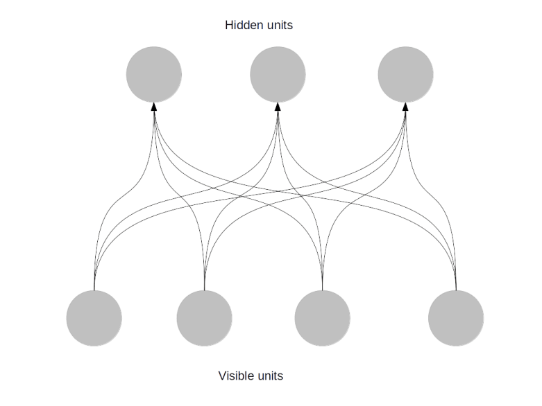
Second, in a restricted Boltzmann machine, certain restrictions on the weights are in effect. Specifically, we only allow hidden units to be connected to visible units and vice versa, so there are no connections between hidden units and no connections between visible units. Effectively, a restricted Boltzmann machine is therefore organised in two layers – one layer containing the hidden units and one layer containing the visible units, as shown below.

What does this imply for the mathematical description of the network? In fact, we will see that this simplifies things considerably. First, corresponding to the differentiation between hidden and visible units, our index set can be written as

$\{ 1, \dots, N \} = I_v \cup I_h$

so that unit i is a hidden unit if i is in the set $I_v$ and a hidden unit if i is in the set $I_h$ . Second, it is common to use 0 and 1 as states instead of -1 and +1. Our state space then splits

$\{ 0, 1\}^N = {\mathcal S} = {\mathcal V} \times \mathcal {H}$

and correspondingly we can write any state as

$s = (v,h)$

where v specifies the state of the visible units and h the state of the hidden units. As only visible units correspond to actual input, the purpose of the training phase is now to adjust the marginal distribution

$P(v) = \sum_h P(v,h) = \frac{1}{Z} \sum_h e^{-\beta E(v,h)}$

such that is it as close as possible to the empirical distribution of the test data.

The expression for the energy also simplifies greatly, as all terms involving only hidden units and only visible units disappear. If we replace the matrix W that contains all connections by a reduced matrix – that we again call W – that only contains the remaining connections between visible and hidden units, we can express the energy as

$E(v,h) = - \sum_{i \in I_v, j \in I_h} W_{ij} v_i h_j$

In addition, we will now also add an explicit bias to both the hidden and visible units, so that our full energy is

$E(v,h) = - \sum_{i \in I_v, j \in I_h} W_{ij} v_i h_j - \sum_i v_i b_i - \sum_j h_j c_j$

Of course the matrix W is now no longer symmetric and not even quadratic (as the number of hidden units will in general not be the same as the number of visible units).

We can now again calculate the update rules as before. First, we write down the likelihood function

$l({\mathcal D} | W) = - \frac{1}{K} \ln P({\mathcal D} | W) = - \frac{1}{K} \sum_k \ln \sum_h e^{-\beta E(v^{(k)},h)}+ \ln Z$

where now $v^{(k)}$ is the k-the sample point corresponding to a set of values for the visible units.

Again we will need the derivatives of this with respect to the weights. For the second term – the logarithm of the partition function – we have already seen in the last post how this works. Recalling the results from this post, we easily find that

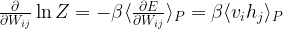
$\frac{\partial}{\partial W_{ij}} \ln Z = - \beta \langle \frac{\partial E}{\partial W_{ij}} \rangle_P = \beta \langle v_i h_j \rangle_P$

so that the derivative is again an expectation value which we could try to approximate using a sample of the model distribution. The first term requires a bit more work. Let us first calculate

$\frac{\partial }{\partial W_{ij}} \ln \sum_h e^{-\beta E(v,h)} = \frac{1}{Z P(v)} \sum_h \frac{\partial }{\partial W_{ij}} e^{-\beta E(v.h)}= - \beta \sum_h \frac{\partial E(v,h)}{\partial W_{ij}} P(h | v)$

But this is again an expectation value, this time it is an expectation value with respect to the conditional distribution of the hidden units given the visible units.

$\frac{\partial }{\partial W_{ij}} \ln \sum_h e^{-\beta E(v,h)} = - \beta \langle \frac{\partial E(v,h)}{\partial W_{ij}} \rangle_{P(\cdot | v)}$

The derivative of the energy with respect to the weights is as above, and we finally obtain the following update rule for the weights:

$\Delta W_{ij} = \lambda \beta \left[ \langle \langle v_i h_j \rangle_{P(\cdot | v)} \rangle_{\mathcal D} - \langle v_i h_j \rangle_P \right]$

Note that the first term is a double expectation value – for each sample $v^{(k)}$ for the visible units, we use the expectation value under the conditional distribution over the hidden units given this value for the visible units.

Now let us start to simplify this expression a bit further, leveraging the restrictions on the geometry of the network. Let us first try to find an expression for the conditional probability

$P(h_j = 1 | v)$

This is in fact easy to calculate in our situation. As the state of a hidden unit does not depend on the other hidden units, but only on the visible units, we find that

$P(h_j = 1 | v)= \sigma(\beta (\sum_i W_{ij} v_i + c_j)) = \sigma(\beta a_j)$

where

$a_j = \sum_i W_{ij} v_i + c_j$

is the activation of the hidden unit j. Using this, we can already simplify the first term in the update rule as follows:

$\langle v_i h_j \rangle_{P(\cdot | v)} = \sum_h P(h | v) v_i h_j = v_i \sum_{h : h_j = 1} P(h | v)$

But this is of course nothing but

$v_i P(h_j = 1 | v)$

so that we eventually find

$\langle v_i h_j \rangle_{P(\cdot | v)} = v_i \sigma (\beta a_j)$

A similar argument works for the second term in the update rule. We have

$\langle v_i h_j \rangle_P = \sum_v \sum_h v_i h_j P(v,h) = \sum_v v_i P(v) \sum_h h_j P(h | v)$

Now the second term sum is again the conditional probability for $h_j$ to be one given v, so that this turns into

$\langle v_i h_j \rangle_P = \sum_v v_i P(v) \sigma(\beta a_j) = \langle v_i \sigma(\beta a_j) \rangle_{P(v)}$

We therefore finally obtain the following simplified update rule.

$\Delta W_{ij} = \beta \left[ \langle v_i \sigma(\beta a_j) \rangle_{\mathcal D} - \langle v_i \sigma(\beta a_j) \rangle_{P(v)} \right]$

Thus again, we see that the gradient is composed of two terms, which we call the positive phase and the negative phase. In each phase, we sample the same expression, once over the data distribution and once over the marginal distribution.

How do we actually calculate these terms? The positive phase is easy – we have written this as an expectation value, but it is nothing but an ordinary sum. For each vector in the sample, we calculate the activation of the hidden unit j, apply the multiplication by $\beta$ and the sigmoid function and multiply the result with the value of the visible unit. So this is in fact an easily calculated analytical expression.

Whereas we have found an analytic expression for the positive phase, there is no obvious analytic expression for the negative phase, so we again need a sampling procedure to calculate this term. At this point, the special structure of the network again helps to make the sampling easier. Suppose we wanted to apply an ordinary Gibbs sampler, where instead of choosing the neuron that we update next randomly, we cycle sequentially through all the neurons. We could then do all the hidden neurons first and then continue with the visible units. Now, as the visible units only depend on the hidden units and vice versa, we could as well update all hidden units in parallel and then all visible units in parallel, using that as in the case of hidden units, the conditional probability for a visible unit to be one can be expressed as

$P(v_i = 1 | h) = \sigma(\beta (\sum_j W_{ij} h_j + b_i))$

This procedure is called Gibbs sampling with block updates. It is also obvious that sampling from the joint distribution $P(v,h)$ in this way and then ignoring the values of the hidden units in this way gives a sampler for the marginal distribution.

Therefore our algorithm to calculate the second term of the update rule would be as follows. We would start with some value for the visible units. Then we would calculate the probability that each hidden unit is on given these values for the visible units and update the hidden units according to this distribution. We would then use the new values for the hidden units, calculate the conditional distribution of the visible units and update the visible units according to this distribution. This would constitute a full Gibbs sampling step. We would repeat this process until convergence is reached and then sample for a few steps to calculate the expectation values above. Plugging this into the update rule and calculating the first term analytically, we would then obtain the needed update for the weights.

So it looks like we are back to our old problem – to calculate one weight update during the gradient descent procedure, we have to run a Gibbs sampler to convergence. Fortunately, it turns out that several approximations exist that make this calculation feasible. Next, we will look at two of these approaches – constrastive divergence and its companion persistent contrastive divergence (PCD). We will then implement both algorithms in Python and try it out, first on a small sample set and then finally on the MNIST data set. But this post has already grown a bit lengthy – so let us save this for the next post in this series.