Boltzmann machines, spin, Markov chains and all that

The image above displays a set of handwritten digits on the left. They look a bit like being sketched on paper by someone in a hurry and then scanned and digitalized, not very accurate but still mostly readable – but they are artificial, produced by a neuronal network, more precisely a so called restricted Boltzmann machine.

On the right hand side, you see the (core part of) the code that has been used to produce this image. These are about forty lines of code, and there is some code around it which is not shown, but stripping off all the comments and boilerplate code, we could probably fit the algorithm into less than fifty lines of code.

I found this contrast always fascinating. Creating something that resembles handwritten digits sounds incredibly complex, but can be done with an algorithm that can  be quenched into a comparatively short program – how does that work? So I started to dig deeper, trying to understand neuronal networks in general and in particular Boltzmann machines – the mathematical foundations, the algorithm and the implementation.

Boltzmann machines are a rather special class of neuronal networks that have a reputation of being hard to train, but are important from a theoretical point of view, being closely related to seemingly remote fields like thermodynamics, statistical mechanics and stochastical processes. That makes them interesting, but also hard to understand. I embarked on that journey a couple of months ago, and I thought it would be nice to create a series of blog posts on this. My current thinking is to have one or two posts on each of the following topics over the next couple of weeks.

• Overview – what are Boltzmann machines (this post)
• Background from statistical mechanics and the Boltzmann distribution
• The Ising model and Gibbs sampling
• Hopfield networks: theory
• Hopfield networks: practice
• From Hopfield networks to Boltzmann machines
• Restricted Boltzmann machines
• Contrastive divergence and PCD
• Implementation with TensorFlow
• Basics of Markov chains
• Finite Markov chains and recurrent Markov chains
• The Metropolis Hasting algorithm

This is a lot of content, and please do not expect to see one post every other day. But maybe I should just start and we will see how it goes….

So let me try to roughly sketch what a Boltzmann machine is. First, it is a neuronal network. As such it is composed of units that can be compared to the neurons in the nervous system. Similar to a neuron, each unit has an input and an output.  The output of a neuron can serve as input for another neuron. In general, every neuron receives inputs from many other neurons and delivers outputs to many other neurons.

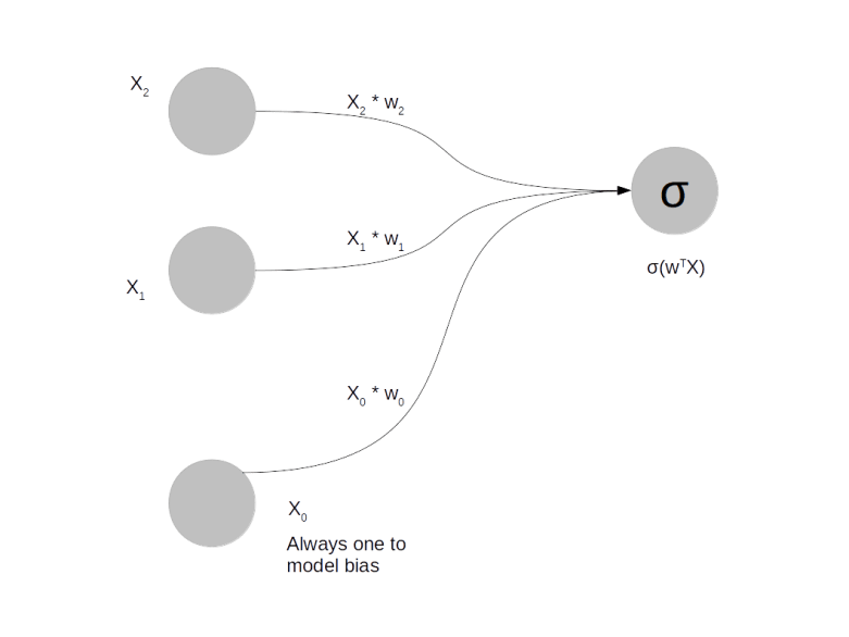
The diagram above shows a very simple neuronal network. It consists of four neurons. The three of them on the left serve as input to the network. Think of them as the equivalent of cells in – say – your visual cortex that are activated by some external stimulus. The cell on the right is the output of the network. Its activation is computed based on the outputs of the neurons on the left and some parameters of the network called the weights which model the strength of the connection between the neurons and which we denote by , as follows.

Here is a function called the activation function and is the vector that is formed by and . There are a few standard choices for the activation function, a common one being the sigmoid function.

How is such a network applied? Let us look at this for a problem which is the “Hello World” of machine learning – recognition of handwritten digits. In that problem, you start with a collection of digitized images of handwritten digits, like those that are known as the MNIST database. These images have 28×28 = 784 pixels. We want to design a neuronal network that can classify these images. Such a network should consequently have 784 input units and 10 output units (bear with me that I did not produce a picture of that network, even though it would probably be fun to do this with Neo4J). We present an image to the network by setting the value of the input unit i to the intensity of pixel i. Our aim is to adjust the weights in such a way that if the image represents digit n, only output n is significantly different from zero. This will allow us to classify unknown images – we simply present the image to the network and then see which output is activated.

But how do we find the correct values for the weights? We need weights that connect each of the ten output units to each of the 784 input units, i.e. we have 7840 weights. Thus we are looking for a point in a 7840 dimensional vector space – not easy. Here the process of training comes into play. We take our set of sample images and present them to the network, with initially randomly chosen weights. The output will then not be what we want, but differ from the target output by an error. That error can be expressed as a function of the weights.  The task is then to find a minimum of the error function, and there are ways to do this, most notably the procedure which is known as gradient descent.

As the name suggests, we need the gradient of the error function for that purpose. Fortunately, for the type of neuronal network that we have sketched so far, the gradient can be computed fairly easily – in fact the activation function is chosen on purpose to make dealing with the derivatives easy. We end up with a comparatively simple training algorithm for this type of network and maybe I will show how a simple implementation in Python in a later post – but for now let us move on to Boltzmann machines.

Boltzmann machines or more precisely restricted Boltzmann machines (RBMs) are also composed of units and weights, but work a bit differently.  There are inputs, which are usually called visible units. But there are no classical outputs. Instead, there is a layer of units that is connected to the visible units and is called hidden units, as shown in the following picture.

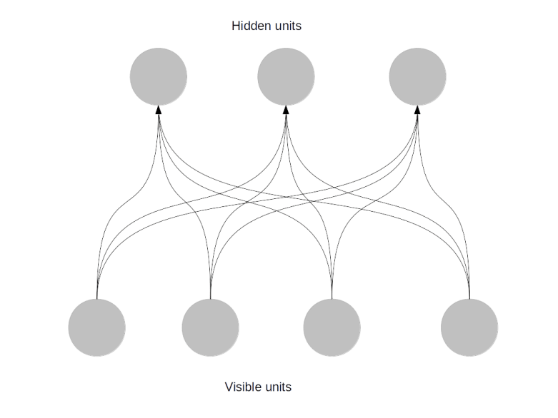
In the example of handwritten digits again, you would again have 784 visible units. However, the hidden units would not obviously correlate with the digit represented by the input. Instead, you would have a more or less arbitrary number of hidden units, say 300.

During training, you present the network one image, again by setting the values of the visible units (the input) to the pixel intensities. You then compute the value of the hidden units – but you do not do this deterministically, but bring in some random element. Roughly speaking, if the combined input to a hidden unit is p, you set the value of the unit to one with probability p. Then this process is repeated, this time starting from the hidden units. This gives you certain values for the visible units. You then compare this value to the original value and try to adjust the weights such that you get as closely as possible to the original input (this is not exactly true and a not very precise description of one of the possible learning algorithms called contrastive divergence, but we will get more precise later on).

If you succeed, you will be able to reconstruct the value of the visible units from the values of the hidden units. But there are less hidden units, so that the network has apparently learned a condensed representation of the input that still captures the essence of the input. In the case of digits, you can visualize the state of the network after training and obtain something like

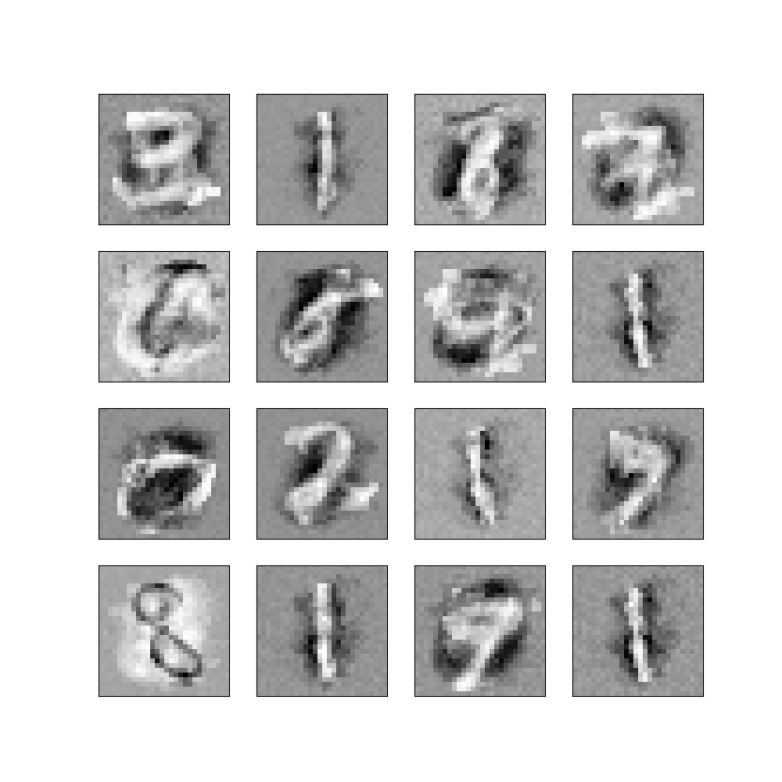
These are visualizations of the weights connected to some of the hidden units of a Bolzmann machine after the training phase. We can see that some of the units have appearantly “learned” some characteristic features of the digits, like the vertical stroke that appears in the digits one and seven. These features can be used for several purposes.

First, we can use the features as input for other neuronal networks. We now have only 300 inputs instead of originally 784, and that might simplify the problem a bit and make the process of training the next network easier.

Or, we could start with some random values for the hidden units and calculate the resulting values of the visible units to create sample images – and in fact this is basically what I have done to produce the samples at the top of this post (using an algorithm called PCD, but we will get to this).

Note that Boltzmann machines differ significantly from the type of neural network that we have considered earlier. One major difference is that to train a Boltzmann machine, you do not need to know the digit that the image represents. At no point have we used the information that the images in our database represent ten different digits – that information was not used in the design of the network nor during the training. This approach to machine learning is called unsupervised learning and is obviously very versatile – you do not have to tell the machine what the structure of the data is, it will detect the features independently.

Second, a Boltzmann machine can not only classify images, but can also create images that resemble a given set of input data. That can be used to reconstruct partially available images or to create new images from scratch – networks with this ability are called generative networks.

The price we have to pay for this is that Boltzmann machines are hard to train. The point is that we can still define some sort of error function, but we cannot easily calculate its gradient – there is no straightforward analytic expression for it that could be evaluated within a reasonable amount of time (if you know statistical physics a bit, that might remind you of the partition function, and that is more than pure coincidence, as I will show you in a later post). So we need to approximate the gradient. Technically, the gradient is an integral

for some known, but complicated function . Even if we cannot find an analytic expression for this, we can try to approximate it. Your first idea might be “Riemann sums”, but it turns out that this is not a good idea, as our function lives in the space of all weights which has a very high dimension. Instead, we will use an approach called Monte Carlo integration where we represent the integral as an expectation value, draw a sample and approximate the expectation value by the sample average. This is where stochastical methods like Markov chains will come into play.  And finally we will see that the behaviour of our network during training has some striking analogies with the behaviour of certain physical systems like solids exposed to a magnetic field at low temperatures, which are described by a model called the Ising model, and learn how techniques that physicists have  developed for this type of problems apply to neuronal networks.

That is it for today – I hope I could give you a rough idea of what is ahead of us. At least I hope that you start to be curious how all this works out – so looking forward to the next post where I will start with some background from physics.