Finite Markov chains

In this post, we will look in more detail into an important class of Markov chains – Markov chains on finite state spaces. Many of the subtleties that are present when studying Markov chains in general state spaces do not appear in the finite case, while most of the key ideas and features of Markov chains are still visible, so this is a good starting point if you want to grasp the key points.

So let us assume that our state space X is finite. For simplicity,  we label our states as where N is the number of states. We also assume that all our points are measurable, i.e we consider our state space as a discrete probability space.

Now consider a sequence of random variables X₀, X₁, …. How can we formalize the idea that X_t+1 depends on X_t in a randomized way?

As so often in probability theory, let us model the dependency as a conditional probability. The conditional probability for X_t+1 to take on a value i given X_t

considered as a function of X_t will assign a conditional probability to each of the states i and for each value of X_t. Therefore we can write this as a matrix

To obtain a time homogeneous Markov chain, we also assume that the matrix K does not depend on the time t. Therefore we define a Markov chain on X to be a sequence of random variables taking values in X with the Markov property saying that for all times t, the conditional distribution for X_t+1 given all previous values only depends on X_t, i.e.

We also require that this conditional probability  is independent of t and is therefore given by a matrix K as in the formula above.

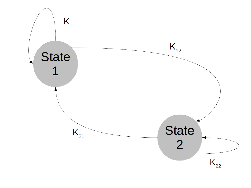
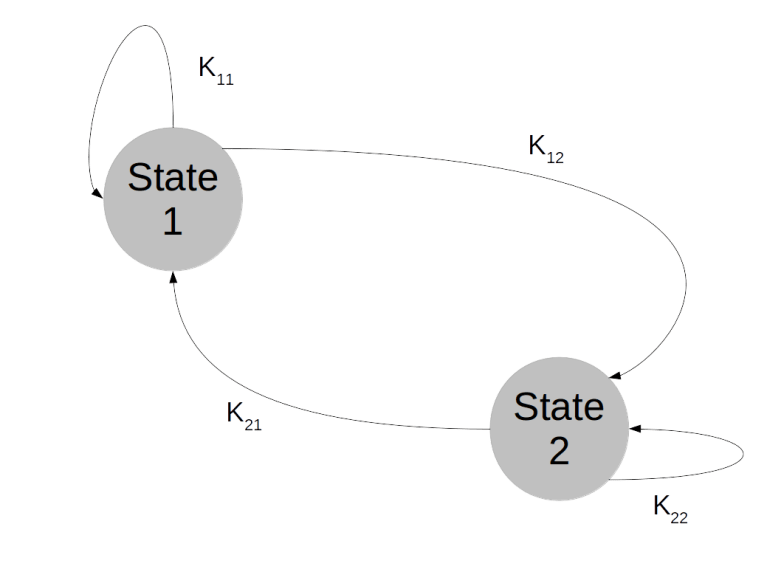
Markov chains on finite state spaces are often visualized as a graph. Suppose, for instance, that our state space contains only two elements: . We can think of the combined values for all times t as a history of states or as a random walk in the state space. The Markov property then means that the probability to transition into a next state does not depend on the full history, but only on the current state – Markov chains do not have a memory.

In our state space with two elements only, the Markov chain is then described by four transition probabilities: the probability to stay in state 1 when the chain is in state 1, the probability to move to state 2 when being in state 1, the probability to stay in state 2 and the probability to move to state 1 after being in state 2. This can be visualized as follows.

Let us now calculate a few probabilities to get an idea for the relevant quantities in such a model. First, suppose that at time 0, the model is in state j with probability . What is the probability to be in state j after one step? Of course we can write

Now, according to the rules of conditional probabilities, we can express the joint probability as follows.

Plugging this into our previous expression and using the definitions of K and , we now obtain

Thus if we think of as a row vector, then the probability after one step is described by the matrix product .

Now let us calculate a slightly different quantity. Assume that we know that a chain starts at j. What is the probability to be at i after two steps? Using once more the rules of conditional probability and the Markov property, we can write

Intuitively, this is very appealing. To get from j to i in two steps, we can take the way via any intermediate state k. To get the total probability, we simply sum up all these different probabilities! If you have ever seen path integrals in quantum mechanics, this idea will look familiar.

Again, we can write this in matrix notation. Each of the conditional probabilities on the right hand side of the expression above is a matrix element, and we find that

so that the probability to get in two steps from j to i is simply given by the elements of the matrix K². Similarly, the n-step transition probabilities are the entries of the matrix Kⁿ.

Let us look at an example to understand what is going on here, which is known as a finite random walk on a circle. Our state space consists of N distinct points which we place arbitrarily on a circle. We then define a Markov chain as follows. We start at some arbitrary point x. In each step, we move along the circle to a neighbored point – one point to the left with probability 1/2 and one point to the right with probability 1/2. By the very definition, the transition probabilities do not change over time and depend only on the current state, so is a finite Markov chain. If we label the points on the circle by , then the transition matrix is given by a matrix of the form (for instance for N=4)

More generally, we can also allow the process to stay where it is with probability 1 – p, where p is then the probability to move, which leads us to the matrix

Let us try to figure out whether the target distribution, given by the matrix Kⁿ for large n, somehow converges.

To see this, we do two numerical experiments. First, we can easily simulate a random walk. Suppose that we have a function draw which accepts a distribution (given by a vector p whose elements add up to one) and draws a random value according to that distribution, i.e. it returns 1 with probability p₀, 2 with probability p₁ and so on. We can then simulate a random walk on the circle as follows.

def simulate_chain(N, p, steps=100, start=5):
    chain = []
    x = start % N
    chain.append(x)
    for i in range(steps):
        x = (x  + draw([p/2.0, 1.0 - p, p / 2.0]) - 2) % N
        chain.append(x)
    return chain

Here N is the number of points on the circle, steps is the number of simulation steps that we run and start is the starting point. The function draw then returns 1 with probability p/2, 3 with probability p/2 and 2 with probability 1 – p. Thus we move with probability p/2 to the right, with probability p/2 to the left and stay were we are with probability 1 – p. If we set p = 0.8, this results in the following transition matrix.

We can visualize the results if we execute a large number of runs and draw histograms of the resulting positions 100, 200, 300, … steps. The result will look roughly like this (for this image, I have used p = 0.8 and N=10):

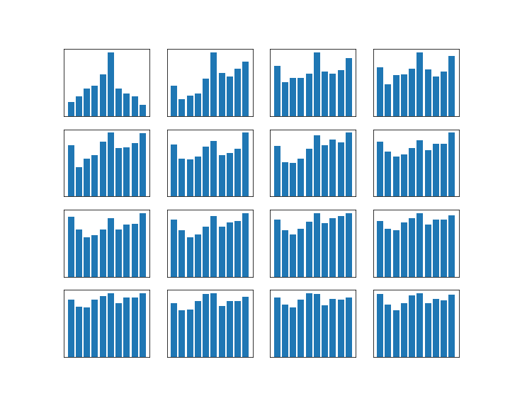
We see that after a few hundred steps, this seems to converge – actually this starts to look very much like a uniform distribution. As we already know that the distribution after n steps is given by the matrix Kⁿ, it makes sense to look at high powers of this matrix as well. To visualize this, I will use a method that I have seen in MacKays excellent book and that works as follows.

Visualizing one row of a matrix is not difficult. We can plot the entries in a two-dimensional diagram, where the x-axis corresponds to the column index and the y-axis corresponds to the value. A flat line is then a row in which all entries have the same value.

To display a full matrix, we use colors – we assign one color to each row index and plot the individual rows as just described. If we do this for the powers of the matrix K with the parameters p = 0.8 and N = 10 (and only chose some rows, for instance 1,4,7, to not run out of colors…) we obtain an image like the one below.

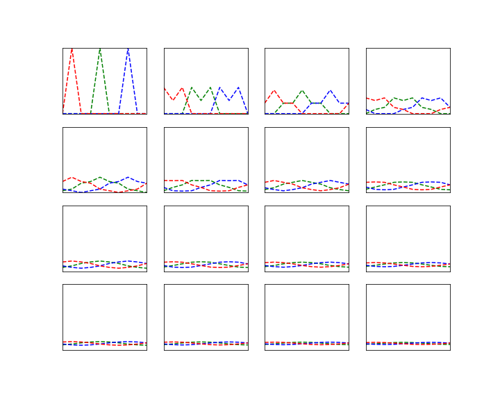
We can clearly see that the powers of the matrix K converge towards a matrix

where all entries in each row seem to have the same value. We have seen that the distribution after n steps assuming an initial distribution described by a row vector is . Therefore the limit distribution is . If we take to be a unit vector, we find that the rows of the matrix do actually represent the limit distribution of all chains that have started at a specific point i of the state space. Therefore the entries in the rows need to sum up to one, and thus, if they are all equal, need to be equal to 1 / N. If you calculate and print out high powers of the matrix K, you will in fact see that they approach the matrix where all entries are 0.1 (as we have chosen N = 10 in this example).

To completes our short introduction into Markov chains. We have seen that Markov chains model stochastic processes in discrete time in which the state at step t+1 depends only on the state at step t and the dependency is given by a function independent of the current time. In finite state spaces, Markov chains are described by a transition matrix K. The i-th row of the matrix Kⁿ is the distribution of chains starting at point i after n steps. Consequently, converge properties of the Markov chains can be related to converge of high powers Kⁿ and the apparatus of linear algebra can be applied.

In the next post, we will learn more about convergence – how it can be made precise, and how we can tell whether a given Markov chain converges. This will then allow us to construct Markov chains that converge towards a given target distribution and use them for sampling.