The EM algorithm and Gaussian mixture models – part I

In the last few posts on machine learning, we have looked in detail at restricted Boltzmann machines. RBMs are a prime example for unsupervised learning – they learn a given distribution and are able to extract features from a data set, without the need to label the data upfront.

However, there are of course many other, by now almost classical, algorithms for unsupervised learning. In this and the following posts, I will explain one of the most commonly applied algorithms in this field, namely the EM algorithm.

As a preparation, let us start with a very fundamental exercise – clustering. So suppose that we are given a data set which we suspect to consist of K clusters. We want to identify these clusters, i.e. to each point in the dataset, we want to assign the number of the cluster to which the point belongs.

More precisely, let us suppose that we are given a set ${\mathcal D} = \{ x_i, \dots, x_N\}$ of points in some euclidian space and a number K of clusters. We want to identify the centre $\mu_i$ of each cluster and then assign the data points x_i to some of the $\mu_j$ , namely to the $\mu_j$ which is closest to x_i. We can encode the assignment of data points to clusters in a matrix R_ij where R_ij = 1 if data point x_i belongs to cluster j with centre $\mu_j$ . Thus each row of R corresponds to a data point and is non-zero in exactly one column, where it is one. This is known as 1-of-K encoding.

For each value of i, the squared distance of x_i to the centre of the cluster to which it is assigned is then given by

$\sum_j R_{ij} \| x_i - \mu_j |^2$

where we note that only one of the summands is different from zero. Assigning the data points to the clusters and positioning the centre points of the clusters then amounts to minimizing the loss function

$l(\mu, R) = \sum_i \sum_j R_{ij} \langle x_i - \mu_j , x_i - \mu_j \rangle$

where the brackets denote the usual euclidean scalar product.

Now let us see how we can optimize this function. For a fixed vector $\mu$ of cluster centers, we can easily minimize R_ij by assigning each data point to the cluster whose center is closest to x_i. Thus we set

$R_{ij} = \begin{cases} 1 & \text{if} \, j = \arg \min \| x_i - \mu_j \|^2 \\ 0 & \text{otherwise} \end{cases}$

Conversely, given a matrix R which we hold fixed, it is likewise easy to minimize $\mu_j$ . As there are no further constraints on $\mu_j$ , we can find the minimum by differentiating the loss function. We find that the derivative is zero if and only if

$0 = \sum_i R_{ij}(x_i - \mu_j)$

holds for all j. Assuming for a moment that each cluster has at least one data point assigned to it, i.e. that none of the columns of R contains zeroes only, we can solve this by

$\mu_j = \frac{\sum_i x_i R_{ij}}{\sum_i R_{ij}}$

which is also easily seen to be a local minimum by taking the second derivative.

Note that this term has an obvious geometric interpretation. The denominator in this expression is the number of data points that are currently assigned to cluster j. The numerator is the sum of all data points assigned to this cluster. Thus the minimum is the mean value of the positions of the data points that are currently assigned to the cluster (a physicist would call this the center of gravity of the cluster). This is the reason why this method is called the k-means algorithm. If no data points are assigned to the cluster, the loss function does not depend on $\mu_j$ and we can choose any value that we want.

The algorithm now works as follows. First, we choose centers $\mu_j$ at will – it is common to use some of the data points for this purpose. Then we assign each data point to a center using the formula for R_ij derived above. We then adjust the center points $\mu_j$ and reallocate the points to the new centers and so forth.

From our discussion above, it is clear that each full iteration of this procedure will reduce the loss function. This does of course not imply that the algorithm converges to a global minimum, as it might get stuck in local minima or saddle points. In practice, the algorithm is executed until the cluster assignments and centers do not change any more substantially or for a given number of steps.

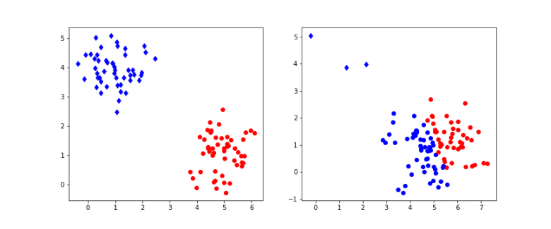
The diagram above shows the result of applying this algorithm to a set of points that is organized in two clusters. To generate the data, 100 samples were drawn from 2-dimensional Gaussian distributions. On the left hand side, half of the the samples were centered at the point (5,1), the other samples at (1,4), and both had standard deviation 0.6. On the right hand side, the same centers were used, but only a small number of samples were drawn from the second distribution which had standard deviation 0.5, whereas most samples came from the first distribution with standard deviation 0.8. Then 10 iterations of the k-means algorithm were applied to the resulting sample set. The points in the sample were then plotted with a color indicating the assignment to clusters resulting from the matrix R. The actual cluster from which the sample was drawn is indicated by the shape – a point is cluster one, a diamond is cluster two.

We see that in the example on the left hand side, the algorithm has correctly assigned all points to their original cluster. For the example on the right hand side, the situation is different – the algorithm did actually assign significantly more points to the blue cluster, i.e. there are many wrong assignments (blue points). This does not change substantially if we increase the number of iterations, even with 100 iterations, we still see many wrong assigments for this example. If you want to reproduce the example and play a bit with the parameters, you can get the sourcecode for a straightforward implementation in Python from my GitHub repository.

The K-means algorithm is very simple and straightforward, but seems to have limitations because it cannot determine the shape of a distribution, only its center. It turns out that K-means is a special case of a broader class of algorithms that we now study, hoping to find more robust algorithms.

In our example, we have generated sample data as a combination of two Gaussian distributions. What if we just change the game and simply assume that our data is of this type? In other words, we assume an underlying probabilistic model for our sample data. Once we have that, we can pull all the tricks that statistical inference can offer – we can calculate maximum likelihood and maximum posterior probability, we can try to determine the posterior or even sample from the model.

Thus let us try to fit our data to a model of the form

$P(x) = \sum_k \pi_k {\mathcal N}(x ; \mu_k, \Sigma_k)$

where ${\mathcal N}(x ; \mu_k, \Sigma_k)$ is a multivariate Gaussian distribution with mean $\mu_k$ and covariance matrix $\Sigma_k$ , i.e.

${\mathcal N}(x ; \mu_k, \Sigma_k) = \frac{1}{\sqrt{(2\pi)^d \det(\Sigma)}} \exp (-\frac{1}{2} \langle x - \mu_k, \Sigma_k^{-1}(x - \mu_k)\rangle)$

and the $\pi_k$ are non-negative real numbers with $\sum_k \pi_k = 1$ .

Let us now see how this equation looks like if we use a 1-of-K encoding. We introduce a random variable Z that takes values in $\{ 0, 1\}^K$ with the additional constraint that only one of the Z_k is allowed to be different from zero. We interpret $\pi_k$ as the probability

$\pi_k = P(Z_k = 1)$

Then

$P(Z = z) = \prod_k \pi_k ^{z_k}$

and we can write

$P(X=x) = \sum_z P(Z=z) P(X=x | Z=z) = \sum_z P(x,z)$

where $P(z)$ is as above and

$P(X = x | Z = z) = \prod_k {\mathcal N}(x ; \mu_k, \Sigma_k)^{z_k}$

This is a very general type of distribution which reflects a common pattern in machine learning, namely the introduction of so called latent or hidden variables. In general, latent or hidden variables are random variables that are a part of the model which cannot be observed, i.e. are not part of the input or the output of the model. We have seen latent variables in action several times – adding hidden units to a neural network introduces latent variables and makes the model much more powerful, the hidden layer of a restricted Boltzmann machine serves as memory to learn features, and latent variables that are used to construct a mixture of Gaussians as above allow us to model a much broader class of distributions than a model with just one Gaussian.

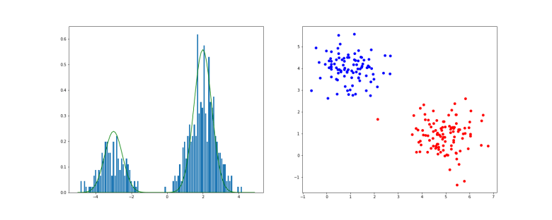
Intuitively, it is also clear how to sample from such a model. In a first step, we sample from Z, in other words we determine the index k randomly according to the distribution given by the $\pi_k$ . Once we have k, we then sample from the conditional distribution $P(X = x | Z = z)$ . As we already have k, this amounts to sampling from the Gaussian distribution ${\mathcal N}(x ; \mu_k, \Sigma_k)$ with mean $\mu_k$ and covariance matrix $\Sigma_k$ .

In the example above, we have first applied this procedure to a one-dimensional Gaussian mixture with K=2. The histogram shows the result of the sampling procedure, the solid lines are the probability density functions of the two individual Gaussian distributions, multiplied by the respective weight. On the right hand side, the result of sampling a Gaussian mixture in two dimensions is displayed (you can download the notebook used to produce this example here).

When we now try to fit this model to the sample data, we again have to calculate the likelihood function and try to maximize it. However, it turns out that the gradient of the likelihood is not so easy to calculate, and it might very well be that there is no closed form solution or that we obtain rather complicated expressions for the gradient. Fortunately, there is an alternative that works for very general models and does not require knowledge of the gradient – the EM algorithm. In the next post, I will present the algorithm in this general setup, before we apply it to our original problem and compare the results with the k-means algorithm.

References

1. C.M. Bishop, Pattern recognition and machine learning, Springer, New York 2006
2. A.P. Dempster, N.M. Laird, D.B. Rubin, Maximum likelihood from incomplete data via the EM-algorithm, Journ. Royal Stat. Soc. Series B. Vol. 39 No. 1 (1977), pp. 1-38

The EM algorithm and Gaussian mixture models – part I

References

Published by christianb93

Leave a Comment Cancel reply

References

Share this:

Like this:

Related

Published by christianb93

Leave a Comment Cancel reply