Python – Page 2 – LeftAsExercise

Asynchronous I/O with Python part II – iterators and generators

As explained in my previous post, historically coroutines in Python have evolved from iterators and generators, and understanding generators is still vital to understanding native coroutines. In this post, we take a short tour through iterators in Python and how generators have traditionally been implemented.

Iterables and iterators

In Python (and in other programming languages), an iterator is an object that returns a sequence of values, one at a time. While in languages like Java, iterators are classes implementing a specific interface, Python iterators are simply classes that have a method __next__ which is supposed to either return the next element from the iterator or raise a StopIteration exception to signal that no further elements exist.

Iterators are typically not created explicitly, but are provided by factory classes called iterables. An iterable is simply a class with a method __iter__ which in turn returns an iterator. Behind the scenes, iterables and iterators are used when you run a for-loop in Python – Python will first invoke the __iter__ of the object to which you refer in the loop to get an iterator and then call the __next__ method of this iterator once for every iteration of the loop. The loop stops when a StopIteration is raised.

This might sound a bit confusing, so let us look at an example. Suppose you wanted to build an object which – like the range object – allows you to loop over all numbers from 0 to a certain limit. You would then first write a class that implements a method __next__ that returns the next value (so it has to remember the last returned value), and then implement an iterable returning an instance of this class.

class SampleIterator:

    def __init__(self, limit):
        self._position = 0
        self._limit = limit

    def __next__(self):
        if self._position < self._limit:
            self._position += 1
            return self._position - 1
        else:
            raise StopIteration

class SampleIterable:

    def __init__(self, limit):
        self._limit = limit

    def __iter__(self):
        return SampleIterator(self._limit)


myIterable = SampleIterable(10)
for i in myIterable:
    print("i = %d" % i)

Often, the same object will implement the __next__ method and the __iter__ method and therefore act as iterable and iterator at the same time.

Note that the iterator typically needs to maintain a state – it needs to remember the state after the last invocation of __next__ has completed. In our example, this is rather straightforward, but in more complex siutations, programmatically managing this state can be tricky. With PEP-255, a new approach was introduced into Python which essentially allows a programmer to ask the Python interpreter to take over this state management – generators.

Generators in Python

The secret sauce behind generators in Python is the yield statement. This statement is a bit like return in that it returns a value and the flow of control to the caller, but with the important difference that state of the currently executed function is saved by Python and the function can be resumed at a later point in time. A function that uses yield in this way is called a generator function.

Again, it is instructive to look at an example. The following code implements our simple loop using generators.

def my_generator(limit=5):
    _position = 0
    while _position < limit:
        yield _position 
        _position += 1

for i in my_generator(10):
    print("i = %d" % i)

We see that we define a new function my_generator which, at the first glance, looks like an ordinary function. When we run this function for the first time, it will set a local variable to set its current position to zero. We then enter a loop to increase the position until we reach the limit. In each iteration, we then invoke yield to return the current position back to the caller.

In our main program, we first call my_generator() with an argument. As opposed to an ordinary function, this invocation does not execute the function. Instead, it evaluates the argument and builds and returns an object called a generator object. This object is an iterator, i.e. it has a __next__ method. When this method is called for the first time, the execution of our function body starts until it hits the first yield statement. At this point, the execution returns to the caller and whatever we yield is returned by the call to __next__. When now __next__ is invoked again, the Python interpreter will restore the current state of the function and resume its execution after the yield. We increase our internal position, enter the loop again, hit the next yield and so forth. This continues until the limit is reached. Then, the function returns, which is equivalent to raising a StopIteration and signals to the caller that the iterator is exhausted.

Instead of using the for loop, we can also go through the same steps manually to see how this works.

generator = my_generator(5)
while True:
    try:
        value = generator.__next__()
        print("Value: %d" % value)
    except StopIteration:
        break

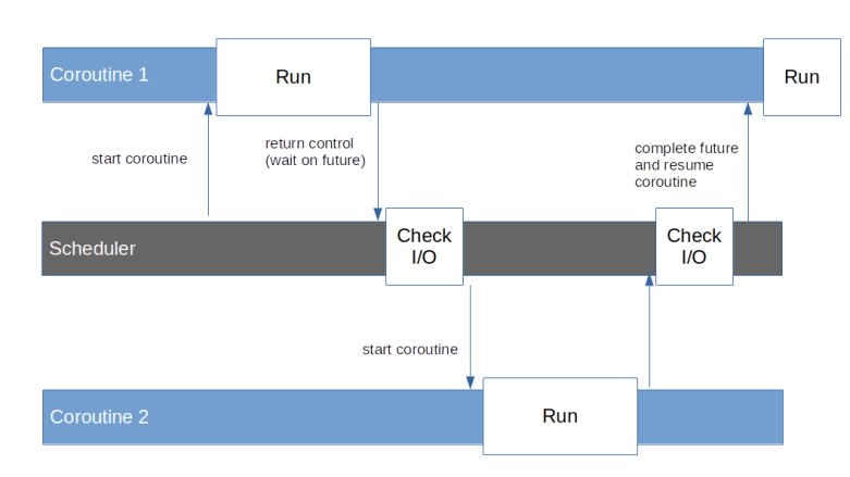
This is already quite close to the programming model of a co-routine – we can start a coroutine, yield control back to the caller and resume execution at a later point in time. However, there are a few points that are still missing and that have been added to Python coroutines with additional PEPs.

Delegation to other coroutines

With PEP-380, the yield from statement was added to Python, which essentially allows a coroutine to delegate execution to another coroutine.

A yield from statement can delegate either to an ordinary iterable or to another generator.

What yield from is essentially doing is to retrieve an iterator from its argument and call the __next__ method of this iterator, thus – if the iterable is a generator – running the generator up to the next yield. Whatever this yield returns will then be yielded back to the caller of the generator containing the yield from statement.

When I looked at this first, I initially was under the impression that if a generator A delegates to generator B by doing yield from B, and B yields a value, control would go back to A, similar to a subroutine call. However, this is not the case. Instead of thinking of a yield from like a call, its better to think of it like a jump. In fact, when B yields a value, this value will be returned directly to the caller of A. The yield from statement in A only returns when B either returns or raises a StopIteration (which is equivalent), and the return value of B will then be the value of the yield from statement. So you might think of the original caller and A as being connected through a pipe through which yielded values are sent back to the caller, and if A delegates to B, it also hands the end of the pipe over to B where it remains until B returns (i.e. is exhausted in the sense of an iterator).

Passing values and exceptions into coroutines

We have seen that when a coroutine executes a yield, control goes back to the caller, i.e. to the code that triggered the coroutine using __next__, and when the coroutine is resumed, its execution continues at the first statement after the yield. Note that yield is a statement and takes an argument, so that the coroutine can hand data back to the caller, but not the other way round. With PEP-342, this was changed and yield became an expression so that it actually returns a value. This allows the caller to pass a value back into the generator function. The statement to do this is called send.

Doing a send is a bit like a __next__, with the difference that send takes an argument and this argument is delivered to the coroutine as result of the yield expression. When a coroutine runs for the first time, i.e. is not resumed at a yield, only send(None) is allowed, which, in general, is equivalent to __next__. Here is a version of our generator that uses this mechanism to be reset.

def my_generator(limit=5):
    _position = 0
    while _position < limit:
        cur = _position
        val = yield cur 
        if val is not None:
            # 
            # We have been resumed due to a send statement. 
            #
            _position = val
            yield val
        else:
            _position += 1

We can now retrieve a few values from the generator using __next__, then use send to set the position to a specific value and then continue to iterate through the generator.

generator = my_generator(20)
assert 0 == generator.__next__()
assert 1 == generator.__next__()
generator.send(7)
assert 7 == generator.__next__()

Instead of passing a value into a coroutine, we can also throw an exception into a coroutine. This actually quite similar to the process of sending a value – if we send a value into a suspended coroutine, this value becomes visible inside the coroutine as the return value of the yield at which the coroutine is suspended, and if we throw an exception into it, the yield at which the coroutine is suspended will raise this exception. To throw an exception into a coroutine, use the throw statement, like

generator = my_generator(20)
assert 0 == generator.__next__()
generator.throw(BaseException())

If you run this code and look at the resulting stack trace, you will see that in fact, the behavior is exactly as if the yield statement had raised the exception inside the coroutine.

The generator has a choice whether it wants to catch and handle the exception or not. If the generator handles the exception, processing continues as normal, and the value of the next yield will be returned as result of throw(). If, however the generator decides to not handle the exception or to raise another exception, this exception will be passed through and will show up in the calling code as if it had been raised by throw. So in general, both send and throw statements should be enclosed in a try-block as they might raise exceptions.

Speaking of exceptions, there are a few exceptions that are specific for generators. We have already seen the StopIteration exception which is thrown if an iterator or generator is exhausted. A similar exception is GeneratorExit which can be thrown into a generator to signal that the generator should complete. A generator function should re-raise this exception or raise a StopIteration so that its execution stops, and the caller needs to handle the exception. There is even a special method close that can be used to close a coroutine which essentially does exactly this – it throws a GeneratorExit into the coroutine and expects the generator to re-raise it or to replace it by a StopIteration exception which is then handled. If a generator is garbage-collected, the Python interpreter will execute this method.

This completes our discussion of the “old-style” coroutines in Python using generator functions and yielding. In the next post, we will move on to discuss the new syntax for native coroutines introduced with Python 3.5 in 2015.

Asynchronous I/O with Python part I – the basics

Though not really new, a programming model commonly known as asynchronous I/O has been attracting a lot of attention over the last couple of years and even influenced the development of languages like Java, Go or Kotlin. In this and the next few posts, we will take a closer look at this model and how it can be implemented using Python.

What is asynchronous I/O?

The basic ideas of asynchronous I/O are maybe explained best using an example from the world of networking, which is at the same time the area where the approach excels. Suppose you are building a REST gateway that accepts incoming connections and forwards them to a couple of microservices. When a new client connects, you will have to make a connection to a service, send a request, wait for the response and finally deliver the response back to the client.

Doing this, you will most likely have to wait at some points. If, for instance, you build a TCP connection to the target service, this involves a handshake during which you have to wait for network messages from the downstream server. Similarly, when you have established the connection and send the request, it might take some time for the response to arrive. While this entire process is n progress, you will have to maintain some state, for instance the connection to the client which you need at the end to send the reply back.

If you do all this sequentially, your entire gateway will block while a request is being processed – not a good idea. The traditional way to deal with this problem has been to use threads. Every time a new request comes in, you spawn a thread. While you have to wait for the downstream server, this thread will block, and the scheduler (the OS scheduler if you use OS-level threads or some other mechanism) will suspend the thread, yield the CPU to some other thread and thus allow the gateway to serve other requests in the meantime. When the response from the downstream server arrives, the thread is woken up, and, having saved the state, the processing of the client’s request can be completed.

This approach works, but, depending on the implementation, creating and running threads can create significant overhead. In addition to the state, concurrently managing a large number of threads typically involves a lot of scheduling, locking, handling of concurrent memory access and kernel calls. This is why you might try a different implementation that entirely uses user-space mechanism.

You could, for instance, implement some user-space scheduler mechanism. When a connection is being made, you would read the incoming request, send a connection request (a TCP SYN) to the downstream server and then voluntarily return control to the scheduler. The scheduler would then monitor (maybe in a tight polling loop) all currently open network connections to downstream servers. Once the connection is made, it would execute a callback function which triggers the next steps of the processing and send a request to the downstream server. Then, control would be returned to the scheduler which would invoke another callback when the response arrives and so forth.

With this approach, you would still have to store some state, for instance the involved connections, but otherwise the processing would be based on a sequence of individual functions or methods tied together by a central scheduler and a series of callbacks. This is likely to be very efficient, as switching between “threads” only involves an ordinary function call which is much cheaper than a switch between two different threads. In addition, each “thread” would only return control to the scheduler voluntarily, implementing a form of cooperative multitasking, and can not be preempted at unexpected points. This of course makes synchronization much easier and avoids most if not all locking, which again removes some overhead. Thus such a model is likely to be fast and efficient.

On the downside, without support from the used programming language for such a model, you will easily end up with a complex set of small functions and callbacks, sometimes turning into a phenomenon known as callback hell. To avoid this, more and more programming languages offer a programming model which supports this approach with libraries and language primitives, and so does Python.

Coroutines and futures

The model which we have described is not exactly new and has been described many years ago. In this model, processing takes place in a set of coroutines. Coroutines are subroutines or functions which have the ability to deliberately suspend their own execution – a process known as yielding. This will save the current state of the coroutine and return control to some central scheduler. The scheduler can later resume the execution of the coroutine which will pick up the state and continue to run until it either completes or yields again (yes, this is cooperative multitasking, and this is where the name – cooperative routines – comes from).

Coroutines can also wait for the result of a computation which is not yet available. Such a result is encapsulated in an object called a future. If, for instance, a coroutine sends a query to a downstream server, it would send the HTTP request over the network, create a future representing the reply and then yield and wait for the completion of this future. Thus the scheduler would gain back control and could run other coroutines. At the same time, the scheduler would have to monitor open network connections, and, when the response arrives, complete the future, i.e. provide a value, and reschedule the corresponding coroutine.

Finally, some additional features would be desirable. To support modularization, it would be nice if coroutines could somehow call each other, i.e. if a coroutine could delegate a part of its work to another coroutine and wait for its completion. We would probably also want to see some model of exception handling. If, for instance, a coroutine has made a request and the response signals an error, we would like to see a way how the coroutine learns about this error by being woken up with an exception. And finally, being able to pass data into an already running coroutines could be beneficial. We will later see that the programming model that Python implements for coroutines supports all of these features.

Organisation of this series

Coroutines in Python have a long history – they started as support for iterators, involved into what is today known as generator-based coroutines and finally turned into the native coroutines that Python supports today. In addition, the asyncio library provides a framework to schedule coroutines and integrate them with asynchronous I/O operations.

Even today, the implementation of coroutines in Python is still internally based on iterators and generators, and therefore it is still helpful to understands these concepts, even if we are mainly interested in the “modern” native coroutines. To reflect this, the remaining posts in this series will cover the following topics.

Iterators and generator-based coroutines
Native coroutines
The main building blocks of the low-level asyncio API – tasks, futures and the event loop
Asynchronous I/O and servers
Building an asynchronous HTTP server from scratch

To follow the programming examples, you will need a comparatively new version of Python, specifically you will need Python 3.7 or above. In case you have an older version, either get the latest version from the Python download page and build it from source, or (easier) try to get a more recent package for your OS (for Ubuntu, for instance, there is the deadsnake PPA that you can use for that purpose).

Learning Kafka with Python – retries and idempotent writes

In the past few posts, we have discussed approaches to implement at-least-once processing on the consumer side, i.e. mechanisms that make sure that every record in the partition is only processed once. Today, we will look at a similar problem on the producer side – how can we make sure that every record is written into the partition only once? This sounds easy, but can be tricky if we need to retry failed message without knowing the exact error that has occured.

The retry problem

In the sample producer that we have looked at in a previous post, we missed an important point – error handling. The most important error that a reliable producer needs to handle is an error when handing over a new record to the broker.

In general, Kafka differentiates between retriable errors, i.e. transient errors like individual packets being lost on the network, and non-retriable errors, i.e. errors like an invalid authorization for which a retry does not make sense. For most transient errors, the client will – under the hood – automatically attempt a retry if a record could not be sent.

Let us take a short look at the Java producer as an example. When a batch of records has been sent to the broker as a ProduceRequest, the response is handled in the method handleProduceResponse. Here, a decision is made whether an automatic retry should be initiated, in which case the batch of records will simply be added to the queue of batches to be sent again. The logic to decide when a retry should be attempted is contained in the method canretry, and in the absence of transactions (see the last section of this post), it will decide to retry if the batch has not timed-out yet (i.e. has been created more than delivery.timeout.ms before), the error is retriable and the number of allowed retries (set via the parameter retries) has not yet been reached. Examples for retriable exceptions are exceptions due to a low number of in-sync replicas, timeouts, connection failures and so forth.

This is nice, but there is a significant problem when using automated retries. If, for instance, a produce request times out, it might very well be that this is only due to a network issue and in the background, the broker has actually stored the record in the partition log. If we retry, we will simply send the same batch of records again, which could lead to duplicate records in the partition log. As these records will have different offsets, there is no way for a consumer to detect this duplicate. Depending on the type of application, this can be a major issue.

If you wanted to solve this on the application level, you would probably set retries to zero, implement your own retry logic and use a sequence number to allow the consumer to detect duplicates. A similar logic referred to as idempotent writes has been added to Kafka with KIP-98 which was implemented in release 0.11 in 2016.

What are idempotent writes?

Essentially, idempotent writes use a sequence number which is added to each record by the producer to allow the broker to detect duplicates due to automated retries. This sequence number is added to a record shortly before it is sent (more precisely, a batch of records receives a base sequence number, and the sequence number of a record is the base sequence number plus its index in the batch), and if an automated retry is made, the exact same batch with the same sequence number is sent again. The broker keeps track of the highest sequence number received, and will not store any records with a sequence number smaller than or equal to the currently highest processed sequence number.

To allow all followers to maintain this information as well, the sequence number is actually added to the partition log and therefore made available to all followers replicating the partitions, so that this data survives the election of a new partition leader.

In a bit more detail, the implementation is slightly more complicated than this. First, it would imply a high overhead to maintain a globally unique sequence number across all producers and partitions. Instead, the sequence number is maintained per producer and per partition. To make this work, producers will be assigned a unique ID called the producer ID. In fact, when a producer that uses idempotent writes starts, it will send an InitPidRequest to the broker. The broker will then assign a producer ID and return it in the response. The producer stores the producer ID in memory and adds it to all records being sent, so that the broker knows from which producer a record originates. Similar to the sequence number, this information is added to the records in the partition log. Note, however, that neither the producer ID nor the sequence number are passed to a consumer by the consumer API.

How does the broker determine the producer ID to be assigned? This depends on whether idempotent writes are used in combination with transactions. If transactions are used, we will learn in the next post that applications need to define an ID called transaction ID that is supposed to uniquely identify a producer. In this case, the broker will assign a producer ID to each transaction ID, so that the producer ID is effectively persisted across restarts. If, however, idempotent writes are used stand-alone, the broker uses a ZooKeeper sequence to assign a sequence number, and if a producer is either restarted or (for instance due to some programming error) sends another InitPidRequest, it will receive a new producer ID. For each new partition assigned to a producer not using transactions, the sequence number will start again at zero, so that the sequence number is only unique per partition and producer ID (which is good enough for our purpose).

Another useful feature of idempotent writes is that a Kafka broker is now able to detect record batches arriving in the wrong order. In fact, if a record arrives whose sequence number is higher than the previously seen sequence number plus one, the broker assumes that records got lost in flight or we see an ordering issue due to a retry and raises an error. Thus ordering is now guaranteed even if we allow more than one in-flight batch.

Trying it out

Time again to try all this. Unfortunately, the Kafka Python client that we have used so far does not (yet) support KIP-98. We could of course use a Java or Go client, but to stick to the idea of this little series to use Python, let us alternatively employ the Python client provided by Confluent.

To install this client, use

pip3 install confluent-kafka==1.4.1

Here I am using version 1.4.1 which was the most recent version at the time when this post was written, so you might want to use the same version. Using the package is actually straightforward. Again, we first create a configuration, then a producer and then send records to the broker asynchronously. Compared to the Kafka Python library used so far, there are a few differences which are worth being noted.

Similar to the Kafka Python library, sends are done asynchronously. However, you do not receive a future when sending as it is the case for the Kafka Python library, but you define a callback directly
To make sure that the callback is invoked, you have to call the poll method of the producer on a regular basis
When you are done producing, you have to explicitly call flush to make sure that all buffered messages are sent
The configuration parameters of the client follow the Java naming conventions. So the bootstrap servers, for instance, are defined by a configuration parameter called bootstrap.servers instead of bootstrap_servers, and the parameter itself is not a Python list but a comma-separated list passed as a string
The base producer class accepts bytes as values and does not invoke a serializer (there is a derived class doing this, but this class is flagged as not yet stable in the API documentation so I decided not to use it)

To turn on idempotent writes, there are a couple of parameters that need to be set in the producer configuration.

enable.idempotence needs to be 1 to turn on the feature
acks needs to be set to “all”, i.e. -1
max.in.flight should be set to one
retries needs to be positive (after all, idempotent writes are designed to make automated retries safe)

Using these instructions, it is now straightforward to put together a little test client that uses idempotent writes to a “test” topic. To try this, bring up the Kafka cluster as in the previous posts, create a topic called “test” with three replicas, navigate to the root of the repository and run

python3 python/idempotent_writes.py

You should see a couple of messages showing the configuration used and indicating that ten records have been written. To verify that these records do actually contain a producer ID and a sequence number, we need to dump the log file on one of the brokers.

vagrant ssh broker1
/opt/kafka/kafka_2.13-2.4.1/bin/kafka-dump-log.sh \
  --print-data-log \
  --files /opt/kafka/logs/test-0/00000000000000000000.log

The output should look similar to the following sample output.

Dumping /opt/kafka/logs/test-0/00000000000000000000.log
Starting offset: 0
baseOffset: 0 lastOffset: 9 count: 10 baseSequence: 0 lastSequence: 9 producerId: 3001 producerEpoch: 0 partitionLeaderEpoch: 0 isTransactional: false isControl: false position: 0 CreateTime: 1589818655781 size: 291 magic: 2 compresscodec: NONE crc: 307611005 isvalid: true
| offset: 0 CreateTime: 1589818655780 keysize: -1 valuesize: 16 sequence: 0 headerKeys: [] payload: {"msg_count": 0}
| offset: 1 CreateTime: 1589818655780 keysize: -1 valuesize: 16 sequence: 1 headerKeys: [] payload: {"msg_count": 1}
| offset: 2 CreateTime: 1589818655780 keysize: -1 valuesize: 16 sequence: 2 headerKeys: [] payload: {"msg_count": 2}
| offset: 3 CreateTime: 1589818655780 keysize: -1 valuesize: 16 sequence: 3 headerKeys: [] payload: {"msg_count": 3}
| offset: 4 CreateTime: 1589818655780 keysize: -1 valuesize: 16 sequence: 4 headerKeys: [] payload: {"msg_count": 4}
| offset: 5 CreateTime: 1589818655780 keysize: -1 valuesize: 16 sequence: 5 headerKeys: [] payload: {"msg_count": 5}
| offset: 6 CreateTime: 1589818655780 keysize: -1 valuesize: 16 sequence: 6 headerKeys: [] payload: {"msg_count": 6}
| offset: 7 CreateTime: 1589818655780 keysize: -1 valuesize: 16 sequence: 7 headerKeys: [] payload: {"msg_count": 7}
| offset: 8 CreateTime: 1589818655780 keysize: -1 valuesize: 16 sequence: 8 headerKeys: [] payload: {"msg_count": 8}
| offset: 9 CreateTime: 1589818655781 keysize: -1 valuesize: 16 sequence: 9 headerKeys: [] payload: {"msg_count": 9}

Here, the third line contains the header of the entire record batch. We see that the batch contains ten records, and we find a producer ID (3001). In each of the records, we also see a sequence number, ranging from 0 to 9.

Transactions

When you read KIP-98, the Kafka improvement proposal with which idempotent writes where introduced, then you realize that the main objective of this KIP is not just to provide idempotent writes, but to be able to handle transactions in Kafka. Here, handling transactions does not mean that Kafka somehow acts as a distributed transaction manager, joining transactions of a relational database. It does, however, mean that writes and reads in Kafka are transactional in the sense that a producer can write records within a transaction, and consumers will either see all of the records written as part of this transaction or none of them.

This makes it possible to model scenarios that occur quite often in business applications. Suppose, for instance, you are putting together an application handling security deposits. When you sell securities, you produce one record which will trigger the delivery of the securities to the buyer, and a second record that will trigger the payment that you receive for them. Now suppose that the first record is written, and them something goes wrong, so that the second record cannot be written. Without transactions, the first record would be in the log and consumers would pick it up, so that the security side of the transaction would still be processed. With transactions, you can abort the transaction, and the record triggering the security transfer will not become visible for consumers.

We will not go into details about transactions in this post, but KIP-98 is actually quite readable. I also recommend that you take a look at this well written blog post on the Confluent pages that provides some more background and additional links.

With that, it is time to close this short series on Kafka and Python. I hope I was able to give you a good introduction into the architecture and operations of a Kafka cluster and a good starting point for own projects. Happy hacking!

Learning Kafka with Python – a deep dive into consumers and rebalancing

In the previous posts, we have already used the Python client to implement Kafka consumers. Today, we will take a closer look at the components that make up a consumer and discuss their inner workings and how they communicate with the Kafka cluster.

High level overview of the consumer

Our discussion will be based on the Kafka Python library, which seems to be loosely modeled after the Java consumer which is part of the official Apache Kafka project, so that the underlying principles are the same. These notes are based on version 2.0.1 of the library, the design might of course change in future versions (and has already changed substantially in the past).

Looking at the code, we see that roughly speaking, the consumer consists of three parts – the actual consumer in the package kafka.consumer, the coordinator which is responsible for talking to the group coordinator and assign partitions in the package kafka.coordinator and the network client in the top-level package which is used by other parts of the library as well. Broken down to the level of modules and classes, the following diagram shows the most important components of the consumer and their relations.

Let us start our discussion with the class on the left hand side of the diagram, the subscription state. This class is used to manage the topics and partitions a consumer has subscribed to as well as the positions of the consumer within these partitions. Note that these positions are not the committed offsets, but are the positions maintained locally (and in-memory) by the consumer that are used to determine the offset that the next fetch will use. Initially, there is no valid position for a newly assigned partition, and the partition is considered fetchable only once a position has been determined.

The second class which is used by the consumer is the fetcher. As the name suggests, this class is in charge for actually fetching data and offsets from the leader of a partition (here, offsets does not refer to committed offsets, but to the valid offsets, i.e. the first and last offset of a partition).

Fetching records from the partition leader typically works asynchronously. As an example, let us consider the method send_fetches. As indicated above, a partition is called fetchable if there is a valid position for it, the partition has not been paused and there are no unfetched records already present in the cache. After creating a list of all fetchable partitions, the send_fetches method then figures out the partition leader and assembles a fetch request. These requests are then sent to the respective partition leader using the client object. This operation returns a future, i.e. a handle which can be used to asynchronously track the progress of the fetch operation. Attached to this future, there is a callback operation. When the records are sent from the partition leader to the consumer, the client object will invoke this callback which will then add the returned records to a queue maintained by the fetcher. From there, it is retrieved when a consumer calls the method fetched_records.

It is in this function where the positions are actually updated, so that the position really reflects the records that have been consumed, not those which have been received by the fetcher but are still in the queue. Note that records are skipped if a partition has become unfetchable in the meantime or if the offset does not match the expected value in the original request.

The following diagram shows a simplified view of how records are fetched (some important details are skipped, for instance the deserialization that takes place when fetched records are removed from the queue and handed over to the consumer).

Coordinating group membership and partition assignments

Apart from fetching records, a core responsibility of the consumer is to manage the membership in a consumer group and to handle assigned partitions. This is done by the coordinator. The coordinator communicates with the group coordinator (which is one dedicated broker per consumer group) to trigger the addition and removal of group members and to balance partitions between group members. In addition, the coordinator is responsible for managing committed offsets.

Looking at the source code of the coordinator, we can see how the process of adding members to the group and assigning partitions works. This process, commonly referred to as rebalancing, typically starts when a consumer invokes the poll method of the coordinator. When this happens, the coordinator will first check whether it needs to join (or rejoin) the group, for instance because the consumer was just started. If yes, the processing in ensure_active_group will first prepare the join process, for instance by committing all offsets if auto-commit is enabled and calling the revoke method of all registered rebalance listeners (conceptually, when a rebalancing starts, all existing members will loose ownership of previously handled partitions and consequently stop processing records so that the group coordinator can reassign partitions freely – there is an ongoing effort known as cooperative rebalancing with the objective to change this).

We then wait until there are no more in-flight requests to the coordinator, and then send a JoinGroupRequest to the group coordinator. The group coordinator (broker) will wait until all members have handed in their requests (see below for more on the timeline) and then determine one member to be the group leader. As part of the JoinGroupResponse, every consumer will be informed about the newly elected leader. The group leader will then perform the actual assignment of partitions to group members (using a configurable assignor). Then, all group members send another request to the group coordinator, called the SyncGroupRequest. In this request, the group leader will inform the group coordinator about the defined partition assignments, and in the response to this message, the partition assignments will be distributed to all group members.

Once the SyncGroupResponse has been received, the method ensure_active_group will invoke _on_join_complete which will in turn trigger a call of the on_partitions_assigned method of all registered rebalance listeners. Note that at this point, all exceptions raised by the listener are swallowed, so exceptions should be caught and handled inside the listener.

This is all nice if our own consumer joins a group, but what happens if another consumer joins? This is where the heartbeat thread comes into play. This is a thread which is running in the background and periodically sending heartbeat messages to the group coordinator (with a frequency determined by the parameter heartbeat_interval_ms). If a rebalancing has been initiated by another member joining or leaving, the heartbeat response will have an error flag set, so that the consumer learns about the start of the rebalancing process. It then sets a flag, which will be evaluated during the next call of the coordinators poll method, which is in turn invoked from the consumers poll loop. If this flag is set, the coordinator will rejoin the group following the process outlined above.

At this point, timing is vital. If a consumer does not call the poll method for a long period of time, it might miss a rebalancing and will forcefully be removed from the group. This again will lead to errors when the consumer tries to commit offsets, which are difficult to handle and almost inevitably lead to duplicate processing. In general, a consumer should invoke the poll method on a regular basis, and there is again a parameter (max_poll_interval_ms) which determines the maximum allowed time between two subsequent invocations of this method.

Indirectly, this parameter also determines how long the group coordinator will wait for members to join the group (it is sent to the group coordinator as part of the join group request). The following diagram shows the typical sequence of events when a new member joins a group and triggers a rebalancing.

The consumers poll loop

After all these preparations, we are now ready to discuss the poll method of the Kafka consumer. In this method (or rather the private method _poll_once), we first use the coordinator and its poll method discussed above to verify that the consumer is part of a group and has partitions assigned and to trigger a rebalancing process if needed. Note that if a rebalancing is needed, this call will block so that it is made sure that we only reach the main part of the consumers poll method after the rebalancing is done.

Next, we will typically have to update all fetch positions. This happens in several steps.

call the method reset_offsets_if_needed of the fetcher. This method will check a flag to see if any offsets need to be reset. If yes, it will retrieve the valid offsets and apply the chosen offset reset strategy
if there are still partitions which do not have a valid position, we call the method refresh_committed_offsets_if_needed of the coordinator which will fetch the committed offsets from the group coordinator
Then, the method update_fetch_positions of the fetcher is invoked which will set the fetch positions of the partitions in question to the committed value

Back in _poll_once, we then check whether the fetcher has any previously obtained records still in its queue. If yes, we immediately return this data (and at the same time initiate a pre-fetch of the next records). Recall that the process of getting these queued records also triggers the update of the position. Then, new fetches are sent, and we poll the client until we either time out or obtain new records which we then return.

Summarizing, the diagram below displays the (slightly simplified) flow of events in case a consumer calls poll (where some calls indicated in the diagram are not made every time, depending on available fetch positions and committed offsets).

From what we have said above, it is now clear that a rebalancing listener is always invoked from within the poll method – which also implies that you should not spend too much time in a rebalance listener and not make any blocking calls.

This completes our short summary of the processing inside the Kafka consumer. With this introduction and using the Java library and the rich comments inside the code, you should now be able to dig deeper into the bits and pieces if needed.

Learning Kafka with Python – implementing a database sink

Very often, either the source or the target of a Kafka based message queue is a classical relational database. Consuming data and using it to update a database table sounds straightforward, but poses a few challenges around reliability and delivery semantics. In this post, we look into two options to realize such an architecture.

The challenge

To illustrate the problem we are aiming to solve, let us suppose that we want to build an application that maintains an account balance. There is a front-end which acts as a Kafka producer and which a customer can use to either deposit money in the account or withdraw money. These transactions are then written into a Kafka topic, and a consumer reads from this topic and updates the balance kept in a relational datastore.

Thus the messages stored in the Kafka topic contains transactions, i.e. changes in the account balance, while the database table we need to maintain contains the actual balance. This is an example of what is called stream / table duality in the world of streaming – the event stream is the source of truth and reflects changes, the database contains the resulting state of the world after all changes have been applied and can at any time be reconstructed from the stream.

When we want to implement his pattern, the crucial part of our design will be to make sure that every message in the queue leads to only one update of the balance, so that no transaction is missed and no transaction is processed twice.

Pattern 1: using a message ID and de-duplication

The first pattern we could use to make this work is to achieve de-duplication based on a unique message ID, which ideally is an integer that is increased with every message. The consumer could then store the sequence number of the last processed message in the database, and could thus detect duplicates.

In a bit more detail, this would work as follows. When the producer processes an action, it first retrieves a unique message ID. This message ID could be created using a database sequence, or – if the used database does not allow for this – it could read a sequence number from a table, increment it by one and update the table accordingly. It would then add this sequence number as a key to the Kafka message.

The consumer would store the latest processed sequence number in the database. When it reads a mesage from Kafka, it uses this number to check whether the message has already been processed before. If not, it updates balance and sequence number in one transaction and then commits the new offset to Kafka.

Let us see how duplicates are handled in this pattern. If, for some reason, the topic contains two messages with the same ID, the consumer will process the first message, increase the latest processed sequence number in the database and commit the new balance. It will then read the duplicate, compare its sequence number against the latest value, detect the duplicate and simply ignore it. Thus the consumer is able to do a de-duplication based on the sequence number.

Unfortunately, this simple pattern has one major disadvantage – it does not work. The problem is that the order of messages is not guaranteed across partitions. Suppose, for instance, that the producer creates the following messages:

Message 1, partition 0
Message 2, partition 1
Message 3, partition 0

Now it might happen that the consumer processes the messages in the order 1,3,2. Thus the consumer would, after having processed message 3, set the highest consumed sequence number to “3” in the database. When now processing message two, our simple duplicate detection algorithm would then classify this message as a duplicate. Thus, to make this work, it is vital that we store the highest processed sequence number by partition and not across all partitions. We could even create the sequence number per partition, which would also remove a possible bottleneck as creating the sequence number would otherwise effectively serialize the producers.

Also note that, as we need to maintain a “last processed” sequence number per partition in a database, we also need to maintain this table if we add new partitions to our topic or remove partitions.

Alternatively, if there is a message ID which is not ordered and increasing with each message, the consumer could store all processed message IDs in a separate database table to keep track of the messages that have already been processed (which, depending on the throughput, might require some sort of periodic cleanup to avoid that the table grows too big).

If the consumer fails after committing the changed balance to the database, but before committing the offset to Kafka, the same mechanism will kick in, as long as we commit the new balance and the updated value of the last processed message in one database transaction. Thus, duplicates can be detected, and we can therefore rely on the standard mechanisms Kafka offers to manage the offset – we could even read entire batches from the topic and use auto-commit to let Kafka manage the offset.

Let us now try out this pattern with the code samples from my repository. To be able to run this, you will have to clone my GitHub repository and follow the instructions in my initial post in this series to bring up your local Kafka cluster. Then, make sure that your current working directory is the root directory of the repository and run the following commands which will install the Python package to access a MySQL database and bring up a Docker based installation of MySQL with a prepared database.

pip3 install mysql-connector-python
./db/createDB.sh

This script will start a Docker container kafka-mysql running MySQL, add a user kafka with a default password to it and create a database kafka for which this user has all privileges. Next, let us run a second script which will (re)-create a Kafka topic transactions with two partitions and initialize the database.

./db/reset.sh

Now we run three Python scripts. The first script is the producer that we have already described, which will simply create ten records, each of which describing a transaction. The second script is our consumer. It will

subscribe to the transactions topic
Read batches of records from the topic
for each record, it will (in one transaction!) update the account balance and the last processed sequence number
commit offsets in Kafka after processing a batch
apply the duplicate detection mechanism outlined above while processing each record

Finally, the third script is a little helper that will (without committing any offsets, so that we can run it over and over again) scan the topic, calculate the expected account balances, retrieve actual account balances from the database and check whether they coincide.

python3 db/producer1.py
python3 db/consumer1.py
python3 db/dump1.py --check

Let us now try to understand how our scripts work if an error occurs. For that purpose, the consumer has a built-in mechanism to simulate random errors between committing to the database and committing offsets to Kafka which is activated using the parameter –error_probability. Let us repeat our test run, but this time we simulate an error with a probability of 20%.

./db/reset.sh && python3 db/producer1.py
python3 db/consumer1.py --error_probability=0.2 --verbose
python3 db/dump1.py --check

You should now see that the consumer processes a couple of messages before our simulated error kicks in, which will make the consumer stop. The check script should detect the difference resulting from the fact that not all messages have been processed. However, when we now restart the script without simulating any errors, we should see that even though there are duplicate records, these records are properly detected and eventually, all records will be processed and the balances will again be correct.

python3 db/consumer1.py --verbose
python3 db/dump1.py --check

Pattern 2: store the consumer offset in the target database

Let us now take a look at an alternative implementation (which is in fact the pattern which you will hit upon first when consulting the Kafka documentation or other sources) – maintaining the offsets in the database altogether. This implementation does not require a sequence number generated by the producer, but is therefore also not able to detect any duplicate messages in case the duplicates originate already in the producer.

The idea behind this pattern is simple. Instead of asking Kafka to maintain offsets for us, the consumer application handles offsets independently and maintains a database table containing offsets and partitions. When a record is processed, the consumer opens a database transaction, updates the account balance and updates the offset in the same transaction. This guarantees that offsets and balances are always in sync.

This sound simple enough, but there are a few subtleties that need to be kept in mind when this is combined with consumer groups, i.e. if Kafka handles partition assignments dynamically. Whenever a partition is assigned to our consumer, we need to make sure that we position the consumer at the latest committed offset before processing any records. Conversely, when an assignment is revoked, we need to commit the current offsets to make sure that they are not lost. This can be implemented using a rebalance listener which is registered when we subscribe to the topic.

To try this out, run the following commands which will first reset the database and the involved topic, run the producer to create a few messages (this time without the additional sequence number) and then run our new consumer to read the messages and update the database.

./db/reset.sh && python3 db/producer2.py
python3 db/consumer2.py 
python3 db/dump2.py --check

The last command, which again checks the updated database table against the expected values, should again show you that expected and actual values in the database match.

It is instructive to try a few more advanced scenarios. You could, for instance, run the producer and then start a consumer which reads the first set of messages produced by the consumer (use the switch –runtime=3600 to make this consumer run for one hour). Then, start a second consumer in a separate terminal window and observe the rebalancing that occurs. Finally, run the producer again and verify that the partition assignment worked and both consumers are processing the messages in their respective partition. And again, you can simulate errors along the way and see how the consumer behaves.

Learning Kafka with Python – producing data

As proud owners of a brand new Kafka installation, we are now ready to explore how applications interact with Kafka. Today, we will look at producers and understand how they write data to Kafka.

Basic design considerations

At first glance, writing data to Kafka sounds easy – connect to a Kafka broker and submit a message. However, there are some basic design considerations that are relevant when building a Kafka producer.

First, we have seen that Kafka stores the data in a topic in multiple partitions, and then each partition has a leader which is responsible for writing messages into the partition. Thus a producer needs to determine to which partition a message should be written and contact the responsible leader for this partition.

Defining the mapping of messages to partitions can be crucial for reliability and scalability of your application. Partitions determine how the application can scale horizontally, and we will learn later that partitions also determine to which extent consumers can scale. In addition, Kafka guarantees message order only within a partition. Specifically, if message A is written to partition before message B is written to the same partition, message A will receive a lower offset than B and will be read first by a (well behaving) consumer. This is no longer true if messages A and B are written to different partitions. Think of partitions as lanes on a highway – there is no guarantee that two cars entering the highway in a certain order but in different lanes will arrive at the destination in the same order.

Often, you will want to use a business entity to partition your data. If you are building a customer facing application, you might want to partition your data by customer group, if you are building a securities processing application the financial instrument might be a good partition criterion, if you are maintaining accounts then the account number might be a good choice and so forth. In other cases, where ordering is not important, you might go for a purely technical criterion.

The next fundamental question we have to figure out is when a message is considered to be successfully written. When the broker has received it? Or when the leader has written the message? Or should we wait until all followers have successfully stored the message? And what if a follower lags behind – should we stop writing messages until the follower has recovered or move on, accepting that we have lost one follower without knowing whether it will recover at a later time?

Kafka does not give a definitive answer to all these questions, but leaves you a choice – put differently, when you create a producer, you can specify its behavior using a variety of options. So let us now see how this is done in Python.

The producer object

Let us now see how a producer can be created using Python. If you have not yet done so, please install the Kafka Python library to be able to run the examples.

pip3 install kafka-python

This series uses version 2.0.1 of the library, if you want to use exactly that version you need to specify that as usual, i.e. run

pip3 install kafka-python==2.0.1

To send messages to Kafka, the first thing we need to do is to create a producer object, i.e. an instance of the class kafka.Producer. The init-method of this class accepts a large number of arguments, but in the most straightforward case, there is exactly one argument bootstrap_servers. This argument is a list of listener URLs, for instance 10.100.0.11:9092, which the producer will use to make an initial connection to a Kafka broker. This list does not need to contain all brokers, in fact one entry will do, but the producer will use this broker to obtain other brokers if needed. It is a good idea to list at least two or three brokers here, in case one broker is temporarily unavailable. So creating a producer could look like this.

import kafka
producer=kafka.KafkaProducer(bootstrap_servers=["broker1:9092", "broker2:9092"])

When started, a Producer will create a separate sender thread which will asynchronously send messages to the brokers. In addition, it will create an internal client which holds the actual connections to the Kafka cluster.

When using an SSL listener, we need a few additional configuration items. Specifically, we need to add the following named parameter when creating a KafkaProducer

ssl_cafile – this is the location of a CA certificate that the client will use to verify the certificate presented by the server
ssl_certfile – this is the location of the client certificate that the client will in turn present to the server when the server requests a certificate
ssl_keyfile – the key matching the client certificate

In order to be bit more flexible when it comes to connecting to different setups, the code examples that we will use in this series read the list of brokers and the SSL configuration from a YAML file config.yaml that the installation script will create in the subdirectory .state of the repository directory. All test scripts accept a parameter –config that you can use to overwrite this default location, in case you want to use your own configuration.

Once we are done using a producer, we should close it using producer.close() to clean up.

Keys and partitions

Once we have a producer in our hands, we can actually start to send messages. This requires only two parameters: the topic (a string) and the payload of the message (a sequence of bytes).

producer.send("test",value=bytes("hello", "utf-8"))

Note that this will create a topic “test” if it does not exist yet, using default values specified in the server configuration (server.properties), so be careful to use this as the default configuration might not be what you want (you can also turn this feature off by setting auto.create.topics.enable to false in server.properties).

Now you might remember from my previous post that a record in Kafka actually consists of a payload and a key. Here, we do not specify a key, so the key will remain empty. But of course, you can define a key for your record by simply adding the named parameter key to the method invocation, like this.

producer.send("test",
        value=bytes("hello", "utf-8"),
        key=bytes("mykey", "utf-8"))

What about partitions? The low-level protocol that a Kafka broker understands expects the client to send a PRODUCE request containing a valid partition ID, so it is up to the client to take this decision. The application programmer can either decide to explictly specify a partition ID (an integer) as an optional parameter to the send method, or let the framework take the decision. In this case, a so-called partitioner is invoked which, based on the value of the key, selects a partition to write to.

An application can set the configuration item partitioner when creating a producer to define a customer partitioner (which is simply a callable object that the producer will invoke). If no partitioner is specified, the default partitioner will be used, which implements the following logic.

If no key is given, the default partitioner will simply distribute the messages randomly across the available partitions
If a key is provided, a hash value of the key will be computed (using a so-called MurmurHash, which will always be an integer. The value of this hash (more precisely, of its last 31 bits) modulo the number of partitions will then determine the partition to use

The important thing to keep in mind is that if you do not provide a key, your message will end up in a random partition. If you do provide a key, then Kafka will guarantee that messages with the same key will go to the same partition and hence be processed in order.

Serialization

In our examples so far, we have passed a sequence of bytes to the send method, both for the key and the value. This is the format that the low-level protocol expects – at the end of the day, keys and values are sent over the wire as a sequence of bytes, and stored as a sequence of bytes.

In many applications, however, you will want to store more complex data types, like JSON data or even objects. So be able to do this with Kafka, you will have to convert your data into a sequence of bytes when sending the data, a process known as serializing.

When creating the producer, you can specify your own serializers for keys and payloads by adding the named parameters key_serializer and value_serializer when creating the producer. Here, a serializer can either be a function which accepts whatever input format you prefer and returns a sequence of bytes, or an instance of the class kafka.serializer.Serializer which has a serialize method which the framework will invoke.

Suppose for instance you wanted to serialize JSON data. Then, you need to provide a serializer which accepts a JSON object and returns a sequence of bytes. For that purpose, we can use the standard json.dumps method to first produce a string, and then encode the string using e.g. UTF-8 to obtain a sequence of bytes. Thus your serializer would look something like

def serialize(data):
    return bytes(json.dumps(data), "utf-8")

and when creating the producer, the call would be something like

producer=kafka.KafkaProducer(..., 
   value_serializer=serialize, ...)

Choosing a reasonable serializer is an important design choice. As Kafka topics are designed to be durable objects, you need to think about things like versioning when the decoding changes as you release new features, and obviously all components of a system need to use matching serializers and de-serializers to be able to exchange data. Many Kafka projects actually use third-party serializers, like Apache Avro or Google’s protobuf.

Acknowledgements

So far, we have seen how we can send messages using the send method of a KafkaProducer object. But in reality, you of course want to know whether your message was successfully send and stored by Kafka.

This leads us to the question at which point a new record can be considered to be committed to a Kafka cluster, i.e. stored and available for consumers. Before getting into this, however, we first have to understand the notion of an in-sync replica.

Recall that Kafka replication works by designating a leader for a partition and zero, one or more followers which constantly ask the leader for new records in the partition and store them in their own copy of the partition log. As the replicas read the records from the leader, the leaders knows which record has been delivered to which follower. The partition can therefore determine whether a replica is out-of-sync, which happens if a follower fails to retrieve the latest message within a defined time frame, or in-sync.

Having enough in-sync replicas is vital for the reliability. If a leader goes down, Kafka has to elect a new leader from the set of available replicas. Of course, choosing an out-of-sync replica to be the new leader would imply that we promote a replica to the master and thus to our new source of truth that not yet replicated all messages that producers have sent to the leader. Thus, making such a replica the new leader results in a loss of records. In some situations, you might still opt to do so, which Kafka allows you if the parameter unclean.leader.election.enable is set to True in the broker configuration.

Now let us come back to the question of when a message sent by a producer will be considered committed. Again, Kafka offers you a choice, governed by the value of the parameter acks of a producer.

When acks = 1 (the default), a message will be considered committed once the leader acknowledges the message. Thus Kafka guarantees that a committed message has been added to the leading partition, but not that it has already been written to one or even all replicas. Note that, as the leader might cache the record in memory, this can lead to data loss if the leader goes down after acknowledging the message, but before a follower has copied it
When acks = -1 (all), a record will be considered committed only once the leader and in addition all in-sync replicas have acknowledged receipt of the message. As long as you have enough in-sync replicas, this gives you a strong guarantee that the message is available on several nodes and thus data loss has become very unlikely
Finally, a value of acks = 0 means that the message will be considered committed once it has been sent over the network, regardless of any acknowledgement from the leader or a follower. This obviously is a very weak guarantee and only reasonable if you have a strong focus on throughtput and can live with a loss of (potentially many) records

When usings acks = all, the number of in-sync replicas is of course vital. To illustrate this, let us assume that you have configured a topic with three replicas, but both followers have become out-of-sync. Now a message will be committed once the leader has written it, meaning that if the leader is lost, the record will be lost as well. To avoid such a scenario, you can set the server property min.insync.replicas. This number determines how many replicas (including the leader) need to be in-sync in order to still accept new messages. Thus if you use, for instance, a topic with a replication factor of three and min.insync.replicas=2 in combinations with acks=-1, then Kafka will guarantee that a message is only reported as committed once the leader and at least one follower have received the record.

Finally, there is one more parameter that is important for the reliability of a producer – max_in_flight_requests_per_connection. A request (which typically contains more than one record to be written) will be considered as in-flight as long as no result – either an acknowledgement or an error – has been received from the broker. If this parameter (which defaults to 5!) is set to a value greater than one, this implies that the producer will not wait for an acknowledgement before sending the next batch. In combination with retries, this can imply that the order in which messages are added to the log is not identical to the order in which they have been sent, and if the producer goes down, in-flight messages night be lost if the broker is not able to process them. Thus set this to one if you need strong guarantees on at-least-one delivery and ordering.

Retries and error handling

Finally, the last important design decision that you need to take when writing a producer is how to deal with errors.

The send method that we are using delivers messages asynchronously to the actual sender and immediately returns. To figure out whether the record was successfully committed, we therefore cannot simply use its return value, but need a different approach. Therefore, the send method returns a handler which can later be used to retrieve the status of the message, a so called Future, or, more precisely, a subclass called FutureRecordMetadata. Once we have this object, we can call its get method with a timeout in seconds to wait for the request to complete. If the request was successful, this method returns a dictionary containing record metadata, otherwise it raises an exception of type kafka.errors.KafkaError. Alternatively, you can also specify callback functions for successful and failed sends.

Note that the producer also has an option to automatically retry failed messages, which can be configured by setting the parameter retries to a value different from zero. In general, however, you should be careful with this as it might conflict with ordering, see the discussion of in-flight requests above.

Testing our producer

After all this theory, it is now time to test our producer. I assume that you have followed my previous post and installed Kafka in three virtual nodes on your PC. Now navigate to the root of the repository and run the following command to create a test topic.

./kafka/bin/kafka-topics.sh \
  --bootstrap-server=$(./python/getBrokerURL.py) \
  --command-config=.state/client_ssl_config.properties \
  --create \
  --topic test \
  --replication-factor 3 \
  --partitions 2

Let us see what this command is doing. The script that we run, kafka-topics.sh, is part of the standard Kafka admin command line tools that are bundled with the distribution. In the second line, we invoke a little Python script that evaluates the configuration in YAML format which our installation procedure has created to determine the URL of a broker, which we then pass to the script. In the third line, we provide a Java properties file containing the SSL parameters to connect to our secured listener.

The remaining switches instruct the tool to create a new topic called “test” with a replication factor of three and two partitions (which, of course, will fail if you have already created this topic in the previous post).

Next, we will run another tool coming with Kafka – the console consumer. This is a simple consumer that will simply subscribe to a topic and dump all records in this topic to the console. To run it, enter

kafka/bin/kafka-console-consumer.sh   \
   --bootstrap-server $(./python/getBrokerURL.py)   \
   --consumer.config .state/client_ssl_config.properties \
   --from-beginning \
   --topic test

Now open an additional terminal, navigate to the root of the repository and run the producer.

python3 python/producer.py

This should print the producer configuration used and the number of messages produced, plus timestamps and the number of seconds and microseconds it took to send all messages. In the first terminal window, in which the consumer is running, you should then see this messages flicker by.

Now let us try out a few things. First, let us create 10000 messages with a set of configurations promising the highest throughput (acks=0, fully asynchronous send, no keys provided, five requests in flight).

python3 python/producer.py \
  --messages=10000 \
  --ack=0

On my PC, producing these 10000 messages takes roughly half a second, i.e. our throughput is somewhere around 20.000 messages per seconds, without any tuning (of course the results will heavily depend on the machine on which you are running this). Next, we produce again 10000 messages, but this time, we use very conservative settings (acks=all, only one message in flight, wait for reply after each request, create and store keys and use them to determine the partition).

python3 python/producer.py \
  --messages=10000 \
  --ack=-1 \
  --max_in_flight_requests_per_connection=1 \
  --wait \
  --create_keys

Obviously, this will be much slower. On my PC, this took roughly 17 seconds, i.e. it is slower by a factor of about 25 than the first run. This hopefully illustrates nicely that Kafka leaves you many choices for trade-offs between performance and availability. Use this freedom with care and make sure you understand the consequences that the various settings have, otherwise you might loose data!

Putting it all together – the send method behind the scenes

Having seen a producer in action, it is instructive to take at a short look at the source code of the Python implementation of KafkaProducer, specifically at its send method. First, the partitions of the topic are retrieved, either from cached metadata or by requesting updated metadata from the server. Then, the key and value are serialized, and the partitioner is invoked which determines the partition to which we write the record.

Next, instead of directly sending the record to the broker, it is appended to an internal buffer using an internal helper class called a RecordAccumulator. If the accumulator signals that the buffer is full, the sender thread is triggered which will then actually transmit the entire batch to the Kafka broker. Finally, the future object is returned.

This completes our discussion of Kafka producers. In the next post, we will learn how we can consume data from Kafka and how consumers, producers and brokers play together.

Learning Kafka with Python – the basics

More or less by accident, I recently took a closer look at Kafka, trying to understand how it is installed, how it works and how the Python API can be used to write Kafka applications with Python. So I decided its time to create a series of blog posts on Kafka to document my learnings and to (hopefully) give you a quick start if you plan to get to know Kafka in a bit more detail. Today, we take a first look at Kafkas architecture before describing the installation in the next post.

What is Kafka?

Kafka is a system for the distributed processing of messages and streams which is maintained as Open Source by the Apache Software foundation. Initially, Kafka was develop by LinkedIn and open-sourced in 2011. Kafka lets applications store data in streams (comparable to a message queue, more on that later), retrieve data from streams and process data in streams.

From the ground up, Kafka has been designed as a clustered system to achieve scalability and reliability. Kafka stores its data on all nodes in a cluster using a combination of sharding (i.e. distributing data across nodes) and replication (i.e. keeping the same record redundantly on several nodes to avoid data loss if a nodes goes down). Kafka clusters can reach an impressive size and throughput and can be employed for a variety of use cases (see for instance this post,this post or this posts to get an idea). Kafka uses another distributed system – Apache ZooKeeper – to store metadata in a reliable way and to synchronize the work of the various nodes in a cluster.

Topics and partitions

Let us start to take a look at some of the core concepts behind Kafka. First, data in Kafka is organized in entities called topics. Roughly speaking, topics are a bit like message queues. Applications called producers write records into a topic which is then stored by Kafka in a highly fault-tolerant and scalable way. Other applications, called consumers, can read records from a topic and process them.

You might have seen similar diagrams before, at least if you have ever worked with messaging systems like RabbitMQ, IBM MQ Series or ActiveMQ. One major difference between these systems and Kafka is that a topic is designed to be a persistent entity with an essentially unlimited history. Thus, while in other messaging systems, messages are typically removed from a queue when they have been read or expired, Kafka records are kept for a potentially very long time (even though you can of course configure Kafka to remove old records from a topic after some time). This is why the data structure that Kafka uses to store the records of a topic is called a log – conceptually, this is like a log file into which you write records sequentially and which you clean up from time to time, but from which you rarely ever delete records programmatically.

That looks rather simple, but there is more to it – partitions. We have mentioned above that Kafka uses sharding to distribute data across several nodes. To be able to implement this, Kafka somehow needs to split the data in a topic into several entities which can then be placed on different nodes. This entity is called a partition. Physically, a partition is simply a directory on one of the nodes, and the data in a partition is split into several files called segments.

Of course, clients (i.e. producers and consumers) do not write directly into these files. Instead, there is a daemon running on each node, called the Kafka broker, which is maintaining the logs on this node. Thus if a producer wants to write into a topic, it will talk to the Broker responsible for the logs on the target node (which depends on the partition, as we will see in later post when we discuss producers in more detail), send the data to the Broker, and the Broker will store the data by appending it to the log. Similarly, a consumer will ask a Broker to retrieve data from a log (with Kafka, consumers pull for data, in contrast to some other messaging systems where data is pushed out to a consumer).

Records in a log are always read and written in batches, not as individual records. A batch consists of some metadata, like the number of records in the batch, and a couple of records. Each record again starts with a short header, followed by a record key and the record payload.

It is important to understand that in Kafka, the record key is NOT identifying a record uniquely. Actually, the record key can be empty and is mainly used to determine the partition to which a record will be written (again, we will discuss this in more detail in the post on producers). Instead, a record is identified by its offset within a partition. Thus if a consumer wants to read a specific record, it needs to specify the topic, the partition number and the offset of the record within the partition. The offset is simply an integer starting at zero which is increased by one for every new record in the topic and serves as a unique, primary key within this partition (i.e. it is not unique across partitions).

Replication, leaders and controllers

Sharding is one pattern that Kafka uses to distribute records across nodes. Within a topic, each partition will be placed on a different node (unless of course the number of nodes is smaller than the number of partitions, in which case some nodes will hold more than one partition). This allows us to scale a Kafka cluster horizontally and to maintain topics that exceed the storage capacity of a single node.

But what if a node goes down? In this case, all data on that node might be lost (in fact, Kafka heavily uses caching and will not immediately flush to disk when a new record is written, so if a node comes down, you will typically lose data even if your file system survives the crash). To avoid data loss in that case, Kafka replicates partitions across nodes. Specifically, for each partition, Kafka will nominate a partition leader and one or more followers. If, for instance, you configure a topic with a replication factor of three, then each partition will have one leader and two followers. All of those three brokers will maintain a copy of the partition. A producer and a consumer will always talk to the partition leader, and when data is written to a partition, it will be synced to all followers.

So let us assume that we are running a cluster with three Kafka nodes. One each node, there is a broker managing the logs on this node. If we now have a topic with two partitions and a replication factor of three, then each of the two partitions will be stored three times, once by the leader and two times on one of the broker nodes which are followers for this topic. This could lead to an assignment of partitions and replicas to nodes as shown below.

If in this situation one of the nodes, say node 1, goes down, then two things will happen. First, Kafka will elect a new leader for partition 0, say node 2. Second, it will ask a new node to create a replica for partition 1, as (even though node 1 was not the leader for partition 1) we now have only one replica for partition 1 left. This process is called partition reassignment.

To support this process, one of the Kafka brokers will be elected as the controller. It is the responsibility of the controller to detect failed brokers and reassign the leadership for the affected partitions.

Producers and consumers

In fact, the process of maintaining replicas is much more complicated than this simple diagram suggests. One of the major challenges is that it can of course happen that a record has been received by the leader and not yet synchronized to all replicas when the leader dies. Will these messages be lost? As often with Kafka, the answer is “it depends on the configuration” and we will learn more about this in one of the upcoming posts.

We have also not yet said anything about the process of consuming from a topic. Of course, in most situations, you will have more than one consumer, either because there is more than one application interested in getting the data or because we want to scale horizontally within an application. Here, the concept of a consumer group comes into play, which roughly is the logical equivalent of an application in Kafka. Within a consumer group, we can have as many consumers as the topic has partitions, and each partition will be read by only one consumer. For consumers, the biggest challenge is to keep track of the messages already read, which is of course essential if we want to implement guarantees like at-least-once or even exactly-once delivery. Kafka offers several mechanisms to deal with this problem, and we will discuss them in depth in a separate post on consumers.

In the next post of this series, we will leave the theory behind for the time being and move on to the installation process, so that you can bring up your own cluster in virtual machines on your PC to start playing with Kafka.

OpenStack Nova – deep-dive into the provisioning process

In the last post, we did go through the installation process and the high-level architecture of Nova, talking about the Nova API server, the Nova scheduler and the Nova agent. Today, we will make this a bit more tangible by observing how a typical request to provision an instance flows through this architecture.

The use case we are going to consider is the creation of a virtual server, triggered by a POST request to the /servers/ API endpoint. This is a long and complicated process, and we try to focus on the main path through the code without diving into every possible detail. This implies that we will skim over some points very briefly, but the understanding of the overall process should put us in a position to dig into other parts of the code if needed.

Roughly speaking, the processing of the request will start in the Nova API server which will perform validations and enrichments and populate the database. Then, the request is forwarded to the Nova conductor which will invoke the scheduler and eventually the Nova compute agent on the compute nodes. We will go through each of these phases in a bit more detail in the following sections.

Part I – the Nova API server

Being triggered by an API request, the process of course starts in the Nova API server. We have already seen in the previous post that the request is dispatched to a controller based on a set of hard-wired routes. For the endpoint in question, we find that the request is routed to the method create of the server controller.

This method first assembles some information like the user data which needs to be passed to the instance or the name of the SSH key to be placed in the instance. Then, authorization is carried out be calling the can method on the context (which, behind the scenes, will eventually invoke the Oslo policy rule engine that we have studied in our previous deep dive). Then the request data for networks, block devices and the requested image is processed before we eventually call the create method of the compute API. Finally, we parse the result and use a view builder to assemble a response.

Let us now see follow the call into the compute API. Here, all input parameters are validated and normalized, for instance by adding defaults. Then the method _provision_instances is invoked, which builds a request specification and the actual instance object and stores these objects in the database.

At this point, the Nova API server is almost done. We now call the method schedule_and_build_instances of the compute task API. From here, the call will simply be delegated to the corresponding method of the client side of the conductor RPC API which will send a corresponding RPC message to the conductor. At this point, we leave the Nova API server and enter the conductor. The flow through the code up to this point is summarized in the diagram below.

Part II – the conductor

In the last post, we have already seen that RPC calls are accepted by the Nova conductor service and are passed on to the Nova conductor manager. The corresponding method is schedule_and_build_instances

This method first retrieves the UUIDs of the instances from the request. Then, for each instance, the private method self._schedule_instances is called. Here, the class SchedulerQueryClient is used to submit an RPC call to the scheduler, which is being processed by the schedulers select_destinations method.

We will not go into the details of the scheduling process here, but simply note that this will in turn make a call to the placement service to retrieve allocation candidates and then calls the scheduler driver to actually select a target host.

Back in the conductor, we check whether the scheduling was successful. It not, the instance is moved into the cell0. If yes, we determine the cell in which the selected host is living, update some status information and eventually, at the end of the method, invoke the method build_and_run_instance of the RPC client for the Nova compute service. At this point, we leave the Nova conductor service and the processing continues in the Nova compute service running on the selected host.

Part III – the processing on the compute node

We have now reached the Nova compute agent running on the selected compute node, more precisely the method build_and_run_instance of the Nova compute manager. Here we spawn a separate worker thread which runs the private method _do_build_and_run_instance.

This method updates the VM state to BUILDING and calls _build_and_run_instance. Within this method, we first invoke _build_resources which triggers the creation of resources like networks and storage devices, and then move on to the spawn method of the compute driver from nova.virt. Note that this is again a pluggable driver mechanism – in fact the compute driver class is an abstract class, and needs to be implemented by each compute driver.

Now let us see how the processing works in our specific case of the libvirt driver library. First, we create an image for the VM by calling the private method _create_image. Next, we create the XML descriptor for the guest, i.e. we retrieve the required configuration data and turn it into the XML structure that libvirt expects. Finally, we call _create_domain_and_network and finally set a timer to periodically check the state of the instance until the boot process is complete.

In _create_domain_and_network, we plug in the virtual network interfaces, set up the firewall (in our installation, this is the point where we use the No-OP firewall driver as firewall functionality is taken over by Neutron) and then call _create_domain which creates the actual guest (called a domain in libvirt).

This delegates the call to nova.virt.libvirt.Guest.create()and then powers on the guest using the launch method on the newly created guest. Let us take a short look at each of these methods in turn.

In nova.virt.libvirt.Guest.create(), we use the write_instance_config method of the host class to create the libvirt guest without starting it.

In the launch method in nova/virt/libvirt/guest.py, we now call createWithFlags on the domain. This is actually a call into the libvirt library itself and will launch the previously defined guest.

At this point, our newly created instance will start to boot. The timer which we have created earlier will check in periodic intervalls whether the boot process is complete and update the status of the instance in the database accordingly.

This completes our short tour through the instance creation process. There are a few points which we have deliberately skipped, for instance the details of the scheduling process, the image creation and image caching on the compute nodes or the network configuration, but the information in this post might be a good starting point for further deep dives.

OpenStack Nova – installation and overview

In this post, we will look into Nova, the cloud fabric component of OpenStack. We will see how Nova is installed and go briefly through the individual components and Nova services.

Overview

Before getting into the installation process, let us briefly discuss the various components of Nova on the controller and compute nodes.

First, there is the Nova API server which runs on the controller node. The Nova service will register itself as a systemd service with entry point /usr/bin/nova-api. Similar to Glance, invoking this script will bring up an WSGI server which uses PasteDeploy to build a pipeline with the actual Nova API endpoint (an instance of nova.api.openstack.compute.APIRouterV21) being the last element of the pipeline. This component will then distribute incoming API requests to various controllers which are part of the nova.api.openstack.compute module. The routing rules themselves are actually hardcoded in the ROUTE_LIST which is part of the Router class and maps request paths to controller objects and their methods.

When you browse the source code, you will find that Nova offers some APIs like the image API or the bare metal API which are simply proxies to other OpenStack services like Glance or Ironic. These APIs are deprecated, but still present for backwards compatibility. Nova also has a network API which, depending on the value of the configuration item use_neutron will either acts as proxy to Neutron or will present the legacy Nova networking API.

The second Nova component on the controller node is the Nova conductor. The Nova conductor does not expose a REST API, but communicates with the other Nova components via RPC calls (based on RabbitMQ). The conductor is used to handle long-running tasks like building an instance or performing a live migration.

Similar to the Nova API server, the conductor has a tiered architecture. The actual binary which is started by the systemd mechanism creates a so called service object. In Nova, a service objects represents an RPC API endpoint. When a service object is created, it starts up an RPC service that handles the actual communication via RabbitMQ and forwards incoming requests to an associated service manager object.

Again, the mapping between binaries and manager classes is hardcoded and, for the Stein release, is as follows.

SERVICE_MANAGERS = {
  'nova-compute': 'nova.compute.manager.ComputeManager',
  'nova-console': 'nova.console.manager.ConsoleProxyManager',
  'nova-conductor': 'nova.conductor.manager.ConductorManager',
  'nova-metadata': 'nova.api.manager.MetadataManager',
  'nova-scheduler': 'nova.scheduler.manager.SchedulerManager',
}

Apart from the conductor service, this list contains one more component that runs on the controller node and use the same mechanism to handle RPC requests (the nova-console binary is deprecated and we use the noVNC proxy, see the section below, the nova-compute binary is running on the compute node, and the nova-metadata binary is the old metadata service used with the legacy Nova networking API). This is the the Nova scheduler.

The scheduler receives and maintains information on the instances running on the individual hosts and, upon request, uses the Placement API that we have looked at in the previous post to take a decision where a new instance should be placed. The actual scheduling is carried out by a pluggable instance of the nova.scheduler.Scheduler base class. The default scheduler is the filter scheduler which first applies a set of filters to filter out individual hosts which are candidates for hosting the instance, and then computes a score using a set of weights to take a final decision. Details on the scheduling algorithm are described here.

The last service which we have not yet discussed is Nova compute. One instance of the Nova compute service runs on each compute node. The manager class behind this service is the ComputeManager which itself invokes various APIs like the networking API or the Cinder API to manage the instances on this node. The compute service interacts with the underlying hypervisor via a compute driver. Nova comes with compute driver for the most commonly used hypervisors, including KVM (via libvirt), VMWare, HyperV or the Xen hypervisor. In a later post, we will go once through the call chain when provisioning a new instance to see how the Nova API, the Nova conductor service, the Nova compute service and the compute driver interact to bring up the machine.

The Nova compute service itself does not have a connection to the database. However, in some cases, the compute service needs to access information stored in the database, for instance when the Nova compute service initializes on a specific host and needs to retrieve a list of instances running on this host from the database. To make this possible, Nova uses remotable objects provided by the Oslo versioned objects library. This library provides decorators like remotable_classmethod to mark methods of a class or an object as remotable. These decorators point to the conductor API (indirection_api within Oslo) and delegate the actual method invocation to a remote copy via an RPC call to the conductor API. In this way, only the conductor needs access to the database and Nova compute offloads all database access to the conductor.

Nova cells

In a large OpenStack installation, access to the instance data stored in the MariaDB database can easily become a bottleneck. To avoid this, OpenStack provides a sharding mechanism for the database known as cells.

The idea behind this is that the set of your compute nodes are partitioned into cells. Every compute node is part of a cell, and in addition to these regular cells, there is a cell called cell0 (which is usually not used and only holds instances which could not be scheduled to a node). The Nova database schema is split into a global part which is stored in a database called the API database and a cell-local part. This cell-local database is different for each cell, so each cell can use a different database running (potentially) on a different host. A similar sharding applies to message queues. When you set up a compute node, the configuration of the database connection and the connection to the RabbitMQ service determine to which cell the node belongs. The compute node will then use this database connection to register itself with the corresponding cell database, and a special script (nova-manage) needs to be run to make these hosts visible in the API database as well so that they can be used by the scheduler.

Cells themselves are stored in a database table cell_mappings in the API database. Here each cell is set up with a dedicated RabbitMQ connection string (called the transport URL) and a DB connection string. Our setup will have two cells – the special cell0 which is always present and a cell1. Therefore, our installation will required three databases.

Database	Description
nova_api	Nova API database
nova_cell0	Database for cell0
nova	Database for cell1

In a deployment with more than one real cell, each cell will have its own Nova conductor service, in addition to a “super conductor” running across cells, as explained here and in diagram below which is part of the OpenStack documentation.

The Nova VNC proxy

Usually, you will use SSH to access your instances. However, sometimes, for instance if the SSHD is not coming up properly or the network configuration is broken, it would be very helpful to have a way to connect to the instance directly. For that purpose, OpenStack offers a VNC console access to running instances. Several VNC clients can be used, but the default is to use the noVNC browser based client embedded directly into the Horizon dashboard.

How exactly does this work? First, there is KVM. The KVM hypervisor has the option to export the content of the emulated graphics card of the instance as a VNC server. Obviously, this VNC server is running on the compute node on which the instance is located. The server for the first instance will listen on port 5900, the server for the second instance will listen on port 5901 and so forth. The server_listen configuration option determines the IP address to which the server will bind.

Now theoretically a VNC client like noVNC could connect directly to the VNC server. However, in most setups, the network interfaces of the compute node are not directly reachable from a browser in which the Horizon GUI is running. To solve this, Nova comes with a dedicated proxy for noVNC. This proxy is typically running on the controller node. The IP address and port number on which this proxy is listening can again be configured using the novncproxy_host and novncproxy_port configuration items. The default port is 6080.

When a client like the Horizon dashboard wants to get access to the proxy, it can use the Nova API path /servers/{server_id}/remote-consoles. This call will be forwarded to the Nova compute method get_vnc_console on the compute node. This method will return an URL, consisting of the base URL (which can again be configured using the novncproxy_base_url configuration item), and a token which is stored in the database as well. When the client uses this URL to connect to the proxy, the token is used to verify that the call is authorized.

The following diagram summarizes the process to connect to the VNC console of an instance from a browser running noVNC.

Client uses Nova API /servers/{server_id}/remote-consoles to retrieve the URL of a proxy
Nova API delegates the request to Nova Compute on the compute node
Nova Compute assembles the URL, which points to the proxy, and creates a token, containing the ID of the instance as well as additional information, and the URL including the token is handed out to the client
Client uses the URL to connect to the proxy
The proxy validates the token, extracts the target compute node and port information, establishes the connection to the actual VNC server and starts to service the session

Installing Nova on the controller node

Armed with the knowledge from the previous discussions, we can now almost guess what steps we need to take in order to install Nova on the controller node.

First, we need to create the Nova databases – the Nova API database (nova_api), the Nova database for cell0 (nova_cell0) and the Nova database for our only real cell cell1 (nova). We also need to create a user which has the necessary grants on these databases.

Next, we create a user in Keystone representing the Nova service, register the Nova API service with Keystone and define endpoints.

We then install the Ubuntu packages corresponding to the four components that we will install on the controller node – the Nova API service, the Nova conductor, the Nova scheduler and the VNC proxy.

Finally, we adapt the configuration file /etc/nova/nova.conf. The first change is easy – we set the value my_ip to the IP of the controller management interface.

We then need to set up the networking part. To enforce the use of Neutron instead of the built-in legacy Nova networking, we set the configuration option use_neutron that we already discussed above to True. We also set the firewall driver to the No-OP driver nova.virt.firewall.NoopFirewallDriver.

The next information we need to provide is the connection information to RabbitMQ and the database. Recall that we need to configure two database connections, one for the API database and one for the database for cell 1 (Nova will automatically append _cell0 to this database name to obtain the database connection for cell 0).

We also need to provide some information that Nova needs to communicate with other Nova services. In the glance section, we need to define the URL to reach the Glance API server. In the neutron section, we need to set up the necessary credentials to connect to Neutron. Here we use a Keystone user neutron which we will set up when installing Neutron in a later post, and we also define some data needed for the metadata proxy that we will discuss in a later post. And finally Nova needs to connect to the Placement service for which we have to provide credentials as well, this time using the placement user created earlier.

To set up the communication with Keystone, we need to set the authorization strategy to Keystone (which will also select the PasteDeploy Pipeline containing the Keystone authtoken middleware) and provide the credentials that the authtoken middleware needs. And finally, we set the path that the Oslo concurrency library will use to create temporary files.

Once all this has been done, we need to prepare the database for use. As with the other services, we need to sync the database schema to the latest version which, in our case, will simply create the database schema from scratch. We also need to establish our cell 1 in the database using the nova-manage utility.

Installing Nova on the compute nodes

Let us now turn to the installation of Nova on the compute nodes. Recall that on the compute nodes, only nova-compute needs to be running. There is no database connection needed, so the only installation step is to install the nova-compute package and to adapt the configuration file.

The configuration file nova.conf on the compute node is very similar to the configuration file on the controller node, with a few differences.

As there is no database connection, we can comment out the DB connection string. In the light of our above discussion of the VNC proxy mechanism, we also need to provide some configuration items for the proxy mechanism.

The configuration item server_proxyclient_address is evaluated by the get_vnc_console of the compute driver and used to return the IP and port number on which the actual VNC server is running and can be reached from the controller node (this is the address to which the proxy will connect)
The server_listen configuration item is the IP address to which the KVM VNC server will bind on the compute host and should be reachable via the server_proxyclient_address from the controller node
the novncproxy_base_url is the URL which is handed out by the compute node for use by the proxy

Finally, there is a second configuration file nova-compute.conf specific to the compute nodes. This file determines the compute driver used (in our case, we use libvirt) and the virtualization type. With libvirt, we can either use KVM or QEMU. KVM will only work if the CPU supports virtualization (i.e. offers the VT-X extension for Intel or AMD-V for AMD). In our setup, the virtual machines will run on top of another virtual machine (Virtualbox), which does only pass through these features for AMD CPUs. We will therefore set the virtualization type to QEMU.

Finally, after installing Nova on all compute nodes, we need to run the nova-manage tool once more to make these nodes known and move them into the correct cells.

Run and verify the installation

Let us now run the installation and verify that is has succeeded. Here are the commands to bring up the environment and to obtain and execute the needed playbooks.

git clone https://www.github.com/christianb93/openstack-labs
cd openstack-labs/Lab4
vagrant up
ansible-playbook -i hosts.ini site.yaml

This will run a few minutes, depending on the network connection and the resources available on your machine. Once the installation completes, log into the controller and source the admin credentials.

vagrant ssh controller
source admin-openrc

First, we verify that all components are running on the controller. To do this, enter

systemctl | grep "nova"

The output should contain four lines, corresponding to the four services nova-api, nova-conductor, nova-scheduler and nova-novncproxy running on the controller node. Next, let us inspect the Nova database to see which compute services have registered with Nova.

openstack compute service list

The output should be similar to the sample output below, listing the scheduler, the conductor and two compute instances, corresponding to the two compute nodes that our installation has.

+----+----------------+------------+----------+---------+-------+----------------------------+
| ID | Binary         | Host       | Zone     | Status  | State | Updated At                 |
+----+----------------+------------+----------+---------+-------+----------------------------+
|  1 | nova-scheduler | controller | internal | enabled | up    | 2019-11-18T08:35:04.000000 |
|  6 | nova-conductor | controller | internal | enabled | up    | 2019-11-18T08:34:56.000000 |
|  7 | nova-compute   | compute1   | nova     | enabled | up    | 2019-11-18T08:34:56.000000 |
|  8 | nova-compute   | compute2   | nova     | enabled | up    | 2019-11-18T08:34:57.000000 |
+----+----------------+------------+----------+---------+-------+----------------------------+

Finally, the command sudo nova-status upgrade check will run some checks meant to be executed after an update that can be used to further verify the installation.

OpenStack Keystone – a deep-dive into tokens and policies

In the previous post, we have installed Keystone and provided an overview of its functionality. Today, we will dive in detail into a typical authorization handshake and take you through the Keystone source code to see how it works under the hood.

The overall workflow

Let us first take a look at the overall process before we start to dig into details. As an example, we will use the openstack CLI to list all existing projects. To better see what is going on behind the scenes, we run the openstack client with the -v command line switch which creates a bit more output than usual.

So, log into the controller node and run

source admin-demorc
openstack -vv project list

This will give a rather lengthy output, so let us focus on those lines that signal that a requests to the API is made. The first API is a GET request to the URL

http://controller:5000/v3

This request will return a list of available API versions, marked with a status. In our case, the result indicates that the stable version is version v3. Next, the clients submits a POST request to the URL

http://controller:5000/v3/auth/tokens

If we look up this API endpoint in the Keystone Identity API reference, we find that this method is used to create and return a token. When making this request, the client will use the data provided in the environment variables set by our admin-openrc script to authenticate with Keystone, and Keystone will assemble and return a token.

The returned data has actually two parts. First, there is the actual Fernet token, which is provided in the HTTP header instead of the HTTP body. Second, there is a token structure which is returned in the response body. This structure contains the user that owns the token, the date when the token expires and the data when the token has been issued, the project for which the token is valid (for a project scoped token) and the roles that the user has for this project. In addition, it contains a service catalog. Here is an example, where I have collapsed the catalog part for better readibility.

Finally, at the bottom of the output, we see that the actual API call to get a list of projects is made, using our newly acquired token and the endpoint

http://controller:5000/v3/projects

So our overall flow looks like this, ignoring some client internal processes like selecting the endpoint (and recovering from failed authorizations, see the last section of this post).

Let us now go through these requests step by step and see how tokens and policies interact.

Creating a token

When we submit the API request to create a token, we end up in the method post in the AuthTokenResource class defined in keystone/api/auth.py. Here we find the code.

token=authentication.authenticate_for_token(auth_data)
resp_data=render_token.render_token_response_from_model(
          token, include_catalog=include_catalog
)

The method authenticate_for_token is defined in keystone/api/_shared/authentication.py. Here, we first authenticate the user, using the auth data provided in the request, in our case this is username, password, domain and project as defined in admin-openrc. Then, the actual token generation is triggered by the call

token=PROVIDERS.token_provider_api.issue_token(
          auth_context['user_id'], 
          method_names, 
          expires_at=expires_at,
          system=system, 
          project_id=project_id, 
          domain_id=domain_id,
          auth_context=auth_context, 
          trust_id=trust_id,
          app_cred_id=app_cred_id, 
         parent_audit_id=token_audit_id)

Here we see an additional layer of indirection in action – the ProviderAPIRegistry as defined in keystone/common/provider_api.py. Without getting into details, here is the idea of this approach which is used in a similar way in other OpenStack services.

Keystone itself consists of several components, each of which provide different methods (aka internal APIs). There is, for instance, the code in keystone/identity handling the core identity features, the code in keystone/assignment handling role assigments, the code in keystone/token handling tokens and so forth. Each of these components contains a class typically called Manager which is derived from the base class Manager in keystone/common/manager.py.

When such a class is instantiated, it registers its methods with the static instance ProviderAPI of the class ProviderAPIRegistry defined in keystone/common/provider_api.py. Technically, registering means that the object is added as attribute to the ProviderAPI object. For the token API, for instance, the the Manager class in keystone/token/provider.py registers itself using the name token_provider_api, so that it is added to the provider registry object as the attribute token_provider_api. Thus a method XXX of this manager class can now be invoked using

from keystone.common import provider_api
provider_api.ProviderAPIs.token_provider_api.XXX()

or by

from keystone.common import provider_api
PROVIDERS = provider_api.ProviderAPIs
PROVIDERS.token_provider_api.XXX()

This is exactly what happens here, and this is why the above line will actually take us to the method issue_token of the Manager class defined in keystone/token/provider.py. Here, we build and populate an instance of the Token class defined in keystone/models/token_model.py and populate it with the available data. We then populate the field token.id where we put the actual token, i.e. the encoded string that will end up in the HTTP header of future requests. This is done in the line

token_id, issued_at =
             self.driver.generate_id_and_issued_at(token)

which calls the actual token provider, for instance the Fernet provider. For a Fernet token, this will eventually end up in the line

token_id=self.token_formatter.create_token(
    token.user_id,
    token.expires_at,
    token.audit_ids,
    token_payload_class,
    methods=token.methods,
    system=token.system,
    domain_id=token.domain_id,
    project_id=token.project_id,
    trust_id=token.trust_id,
    federated_group_ids=token.federated_groups,
    identity_provider_id=token.identity_provider_id,
    protocol_id=token.protocol_id,
    access_token_id=token.access_token_id,
    app_cred_id=token.application_credential_id
)

calling the token formatter which will do the low level work of actually creating and encrypting the token. The token ID will then be added to the token data structure, along with the creation time (a process known as minting) before the token is returned up the call chain.

At this point, the token does not yet contain any role information and no service catalog. To enrich the token by this information, it is rendered by calling render_token defined in keystone/common/render_token.py. Here, a dictionary is built and populated with data including information on role, scope and endpoints.

Note that the role information in the token is dynamic, in fact, in the Token class, the property decoration is used to divert access to the roles property to a method call. Here, we receive the scope information and select and return only these roles which are bound to the respective domain or project if the token is domain scoped or project scoped. When we render the token, we access the roles attribute and retrieve the role information from the method bound to it.

Within this method, an additional piece of logic is implemented which is relevant for the later authorization process. Keystone allows an administrator to define a so-called admin project. Any user who authenticates with a token scoped to this special project is called a cloud admin, a special role which can be referenced in policies. When rendering the token, the project to which the token refers (if it its project scoped) is compared to this special project, and if they match, an additional attribute is_admin_project is added to the token dictionary.

Finally, back in the post method, we build the response body from the token structure and add the actual token to the response header in the line

response.headers['X-Subject-Token'] = token.id

Here is a graphical overview on the process as we have discussed it so far.

The key learnings from the code that we can deduce so far are

The actual Fernet token contains a minimum of information, like the user for whom the token is issued and – depending on the scope – the Ids of the project or domain to which the token is scoped
When a token is requested, the actual Fernet token (the token ID) is returned in the response header, and an enriched version of the token is added in the response body
This enrichment is done dynamically using the Keystone database, and the enrichment will only add the roles to the token data that are relevant for the token scope
There is a special admin project, and a token scoped to this project implies the cloud administrator role

Using the token to authorize a request

Let us now see what happens when a client uses this token to actually make a request to the API – in our example, this happens when the openstack client makes the actual API call to the endpoint http://controller:5000/v3/projects.

Before this request is actually dispatched to the business logic, it passes through the WSGI middleware. Here, more precisely in the class method AuthContextMiddleware.process_request defined in the file keystone/server/flask/request_processing/middleware/auth_context.py, the token is retrieved from the field X-Auth-Token in the HTTP header of the request (here we also put the marker field is_admin into the context when an admin_token is defined in the configuration and equal to the actual token). Then the process_request method of the superclass is called which invokes fetch_token (of the derived class!). Here, the validate_token method of the token provider is called which performs the actual token validation. Finally, the token is again rendered as above, thereby adding the relevant roles dynamically, and put as token_reference in the request context (this happens in the method fill_context respectively _keystone_specific_values of the middleware class).

At this point, it is instructive to take a closer look at the method that actually selects the relevant roles – the method roles of the token class defined in keystone/models/token_model.py. If you follow the call chain, you will find that, to obtain for instance all project roles, the internal API of the assignment component is used. This API returns the effective roles of the user, i.e. roles that include those roles that the user has due to group membership and roles that are inherited, for instance from the domain-level to the project level or down a tree of subprojects. Effective roles also include implied roles. It is important to understand (and reasonable) that it is the effective roles that enter a token and are therefore evaluated during the authorization process.

Once the entire chain of middleware has been processed, we finally reach the method _list_projects in keystone/api/projects.py. Close to the start of this method, the enforce_call method of the class RBACEnforcer in keystone/common/rbac_enforcer/enforcer.py. When making this call, the action identity:list_projects is passed as a parameter. In addition, a parameter called target is passed, a dictionary which contains some information on the objects to which the API request refers. In our example, as long as we do not specify any filters, this dictionary will be empty. If, however, we specify a domain ID as a filter, it will contain the ID of this domain. As we will see later, this allows us to define policies that allow a user to see projects in a specific domain, but not globally.

The enforce_call method will first make a couple of validations before it checks whether the request context contains the attribute is_admin. If yes, the token validation is skipped and the request is always allowed- this is to support the ADMIN_TOKEN bootstrapping mechanism. Then, close to the bottom of the method, we retrieve the request context, instantiate a new object and calls its _enforce method which essentially delegates the call to the Oslo policy rules engine and its Enforcer class, more precisely to the enforce method of this class.

As input, this method receives the action (identity:list_projects in our case), the target of the action, and the credentials, in the form of the Oslo request context, and the processing of the rules starts.

Again, let us quickly summarize what the key take aways from this discussion should be – these points actually apply to most other OpenStack services as well.

When a request is received, the WSGI middleware is responsible for validating the token, retrieving the additional information like role data and placing it in the request context
Again, only those roles are stored in the context which the user has for the scope of the token (i.e. on project level for project-scoped token, on the domain level for domain-scoped token and on the system level for system-scoped token)
The roles in the token are effective roles, i.e. taking inheritance into account
The actual check against the policy is done by the Oslo policy rule engine

The Oslo policy rule engine

Before getting into the details of the rule engine, let us quickly summarize what data the rule engine has at its disposal. First, we have seen that it receives the action, which is simply a string, identity:list_projects in our case. Then, it has information on the target, which, generally speaking, is the object on which the action should be performed (this is less relevant in our example, but becomes important when we modify data). Finally, it has the credentials, including the token and role information which was part of the token and is now stored in the request context which the rule engine receives.

The engine will now run this data through all rules which are defined in the policy. Within the engine, a rule (or check) is simply an object with a __call__ method, so that they can be treated and invoked like a function. In the module _checks.py, a few basic checks are defined. There are, for instance, simple checks that always return true or false, and their checks like AndCheck and OrCheck which can be used to build more complex rules from basic building blocks. And there are other checks like the RoleCheck which checks whether a certain role is present in the credentials, which, as we know from the discussion above, is the case if the token use to authorize contains this role, i..e if the user who is owning the token has this role with respect to the scope of the token.

Where do the rules come from that are processed? First, note that the parameter rule to the enforce method does, in our case at least, contain a string, namely the action (identity:list_projects). To load the actual rules, the method enforce will first call load_rules which loads rules from a policy file, at which we will take a look in a second. Loading the policy file will create a new instance of the Rules class, which is a container class to hold a set of rules.

After loading all rules, the following line in enforce identifies the actual rule to be processed.

to_check = self.rules[rule]

This looks a bit confusing, but recall that here, rule actually contains the action identity:list_projects, so we look up the rule associated with this action. Finally, the actual rule checking is done by invoking the _check methods of the _checks module.

Let us now take a closer look at the policy files themselves. These files are typically located in the /etc/XXX subdirectory, where XXX is the OpenStack component in question. Samples files are maintained by the OpenStack team. To see an example, let us take a look at the sample policy file for Keystone which was distributed with the Rocky release. Here, we find a line

identity:list_projects": "rule:cloud_admin or rule:admin_and_matching_domain_id",

This file is in JSON syntax, and this line defines a dictionary entry with the action identity:list_projects and the rule rule:cloud_admin or rule:admin_and_matching_domain_id. The full syntax of the rule is explained nicely here or in the comments at the start of policy.py. In essence, in our example, the rule says that the action is allowed if either the user is a cloud administrator (i.e. an administrator the the special admin project or admin domain which can be configured in the Keystone configuration file) or is an admin for the requested domain.

When I first looked at the policy files in my test installation, however, which uses the Stein release, I was more than confused. Here, the rule for the action identity:list_projects is as follows.

"identity:list_projects": "rule:identity:list_projects"

Here we define a rule called identity:list_projects for the action with the same name, but where is this rule defined?

The answer is that there is a second source of rules, namely software defined rules (which the OpenStack documentation calls policy-in-code) which are registered when the enforcer object is created. This happens in the _enforcer method of the RBACEnforcer when a new enforcer is created. Here we call register_rules which creates a list of rules by calling the function list_rules define in the keystone/common/policies module which returns a list of sofware-defined rules, and registers these rules with the Oslo policy enforcer. The rule we are looking for, for instance, is defined in keystone/common/policies/project.py and looks as follows.

policy.DocumentedRuleDefault(
        name=base.IDENTITY % 'list_projects',
        check_str=SYSTEM_READER_OR_DOMAIN_READER,
        scope_types=['system', 'domain'],
        description='List projects.',
        operations=[{'path': '/v3/projects',
                     'method': 'GET'}],
        deprecated_rule=deprecated_list_projects,
        deprecated_reason=DEPRECATED_REASON,
        deprecated_since=versionutils.deprecated.STEIN),

Here we see that the actual rule (in the attribute check_str) has now changed compared to the Rocky release, and allows access if either the user has the reader role on the system level or has the reader role for the requested domain. In addition, there is a deprecated rule for backwards compatibility which is OR’ed with the actual rule. So the rule that really gets evaluated in our case is

(role:reader and system_scope:all) or (role:reader and domain_id:%(target.domain_id)s) or rule:admin_required

In our case, asking OpenStack to list all projects, there is a further piece of magic involved. This becomes visible if you try a different user. For instance, we can create a new project demo with a user demo who has the reader role for this project. If you now run the OpenStack client again to get all projects, you will only see those projects for which the user has a role. This is again a bit confusing, because by what we have discussed above, the authorization should fail.

In fact, it does, but the client is smart enough to have a plan B. If you look at the output of the OpenStack CLI with the -vvv flag, you will that a first request is made to list all projects which fails, as expected. The client then tries a second request, this time using the URL /users//projects to get all projects for that specific user. This call ends up in the method get of the class UserProjectsResource defined in keystone/api/users.py which will list all projects for which a specifc user has a role. Here, a call is made with a different action called identity:list_user_projects, and the rule for this action allows access if the user making the request (i.e. the user data from the token) is equal to target user (i.e. the user ID specified in the request). Thus this final call succeeds.

These examples are hopefully sufficient to demonstrate that policies can be a tricky topic. It is actually very instructive to add debugging output to the involved classes (the Python source code is on the controller node in /usr/lib/python3/dist-packages, do not forget to restart Apache if you have made changes to the code) to print out the various structures and trace the flow through the code. Happy hacking!