NMR based quantum computing: gates and state preparation

In my last post on NMR based quantum computing, we have seen how an individual qubit can be implemented based on NMR technology. However, just having a single qubit is of course not really helpful – what we are still missing is the ability to initialize several qubits and to realize interacting quantum gates. These are the topics that we will discuss today.

The physics and mathematics behind these topics is a bit more involved, and I will try to keep things simple. In case you would like to dive more deeply into some of the details, you might want to take a look at my notes on GitHub as well as the references cited there.

Pseudo-pure states

In quantum computing, we are typically manipulating individual qubits which are initially in a pure state. In an NMR probe, however, we usually have a state which is very far from being a pure state. Instead, we typically deal with highly mixed states, and it appears to be impossible to prepare all spins in an NMR probe in the same, well defined pure state. So we first need to understand how the usual formalism of quantum computing – expressed in terms of qubits being in pure states which are subject to unitary operations – relates to the description of an NMR experiment in terms of density matrices and mixed states.

The formalism that we will now describe is known as the formalism of pseudo-pure states. These are states that are described by a density matrix of the form

\rho = \frac{1}{2^N}(1-\epsilon) + \epsilon |\psi \rangle \langle \psi |

with a pure state |\psi \rangle. Here, N is the number of spins, and the factor 1/2N has been inserted to normalize the state. This density matrix describes an ensemble for which almost all molecules are in purely statistically distributed states, but a small fraction – measured by \epsilon – of them are in a pure state. The second term in this expression is often called the deviation and denoted by \rho_\Delta.

Why are these states useful? To see this, let us calculate the time evolution of this state under a unitary matrix U. In the density matrix formalism, the time evolution is given by conjugation, and a short calculation shows that

U(t) \rho U(t)^{-1} = \frac{1}{2^N} (1-\epsilon) + \epsilon |U(t) \psi \rangle \langle U(t) \psi |

Thus the result is again a pseudo-pure state. In fact, it is the pseudo-pure state that corresponds to the pure state U|\psi \rangle. Similarly, one can show that if A is an observable, described by a hermitian matrix (which, for technical reasons, we assume to be traceless), then the expectation value of A evaluated on |\psi \rangle – which is the result a measurement would yield in the pure state formalism – is, up to a constant, the same as the result of a measurement of A on an ensemble prepared in the pure state corresponding to |\psi \rangle!

Using these relations, we can now translate the typical process of a quantum computation as expressed in the standard, pure state formalism, into NMR terminology as follows.

  • The process of initializing a quantum computer into an initial state |\psi \rangle corresponds to putting the NMR probe into the corresponding pseudo-pure state with \rho_{\Delta} \sim |\psi \rangle \langle \psi|
  • If the quantum algorithm is described as a unitary operator U (typically presented as a sequence of gates Ui), we apply the same unitary operator to the density matrix, i.e. we realize the gates as an NMR experiment
  • We then measure the macroscopic quantity A which will give us – up to a factor – the result of the calculation

This is nice, but how do we prepare these states? Different researchers have come up with different techniques to do this. One of the ideas that is commonly applied is averaging. This is based on the observation that the state at thermal equilibrium is a pseudo-pure state up to an error term. This error term can be removed by averaging over many instances of the same experiment (while somehow shuffling the initial states around using a clever manipulation). So we first let the probe settle down, i.e. prepare it in a thermal state (which can even be at room temperature). We then run our quantum algorithm and measure. Next, we re-initialize the system, apply a certain transformation and re-run the algorithm. We repeat this several times, with a prescribed set of unitary transformations that we apply in each run to the thermal equilibrium state before running the quantum algorithm. At the end, we add up all our results and take the average. It can be shown that these initial “shuffling transformations” can be chosen such that the difference between the thermal state and the pseudo-pure state cancels out.

Quantum gates

Having this result in place, we now need to understand how we can actually realize quantum gates. In the last post, we have already seen that we can use RF-pulses to rotate the state of an NMR qubit on the Bloch sphere, which can be used to realize single qubit gates. But how do we realize two-qubit gates like the CNOT gate? For that purpose, we need some type of interaction between two qubits.

Now, in reality, any two molecules in an NMR probe do of course interact – by their electric and magnetic fields, by direct collision and so forth. It turns out that in most circumstances, all but one type of coupling called the J-coupling can be neglected. This coupling is an indirect coupling – the magnetic moment created by a nuclear spin interacts with the electric field of an electron, which in turn interacts with the magnetic moment of a different nuclear spin. In the Hamiltonian – in a rotating frame – the J-coupling contributes a term like

\frac{2 \pi}{\hbar} J_{12} I^1_z I^2_z

where J12 is a coupling constant. This term introduces a correlation between the two nuclear spins, similar to an additional magnetic field depending on the state of the second qubit. The diagram below is the result of a simulation of an initial state to which J-coupling is applied and demonstrates that the J-coupling manifests itself in a splitting of peaks in an NRM diagram.

TwoCoupledNucleiNMRSignalFFT

An NMR diagram is the result of a Fourier transform, so an additional peak corresponds to a slow, additional rotation of the two spin polarizations around each other.

Let us take a closer look at this. If we apply a free evolution under the influence of J-coupling over some time t, it can be shown – again I refer to my notes on GitHub for the full math – that the time evolution is given by the operator

U = \cos (\frac{\pi J_{12}}{2} t) -i \sigma_z^1 \sigma_z^2 \sin (\frac{\pi J_{12}}{2}  t)

If we choose t such that

\frac{\pi J_{12}}{2} t = \frac{\pi}{4}

and combine this time evolution with rotations around the z-axis of both qubits, we obtain the following transformation, expressed as a matrix

R_{z^2}(-\frac{\pi}{2}) R_{z^1}(-\frac{\pi}{2}) U =  \frac{1+i}{\sqrt{2}} \begin{pmatrix} 1 & & & \\ & 1 & & \\ & & 1 & \\ & & & -1  \end{pmatrix}

Technically, this transformation is the result of letting the system evolve under the influence of J-coupling for the time t and then applying two sharp RF pulses, one at resonance with the first qubit and one at resonance with the second qubit, timed such that they correspond to a rotation on the Bloch sphere around the z-axis with angle \pi / 2. The matrix on the right hand side of this equation represents a two-qubit transformation known as the controlled phase gate. This gate corresponds to applying a phase gate to the second qubit, conditional on the state of the first qubit.

This already looks very similar to a CNOT gate, and in fact it is – one can easily show that the phase gate is equivalent to the CNOT gate up to single qubit operations, more precisely these two gates are related by

C_{NOT} = (I \otimes H) C_{PHASE} (I \otimes H)

where I is the identity and H is the Hadamard gate. As single qubit operations can be realized by RF pulses, this shows that a CNOT gate can be realized by a free evolution under the J-coupling, framed by sequences of RF pulses. This, together with single qubit gates, gives us a universal gate set.

This completes our short deep dive into NMR based quantum computing. Historically, NMR based quantum computers were among the first fully functional implementations of (non error-corrected) universal quantum computers, but have come a bit out of fashion in favor of other technologies. At the time of writing, most of the large technology players focus on a different approach – superconducting qubits – which I will cover in the next couple of posts on quantum computing.

Kubernetes services and load balancers

In my previous post, we have seen how we can use Kubernetes deployment objects to bring up a given number of pods running our Docker images in a cluster. However, most of the time, a pod by itself will not be able to operate – we need to connect it with other pods and the rest of the world, in other words we need to think about networking in Kubernetes.

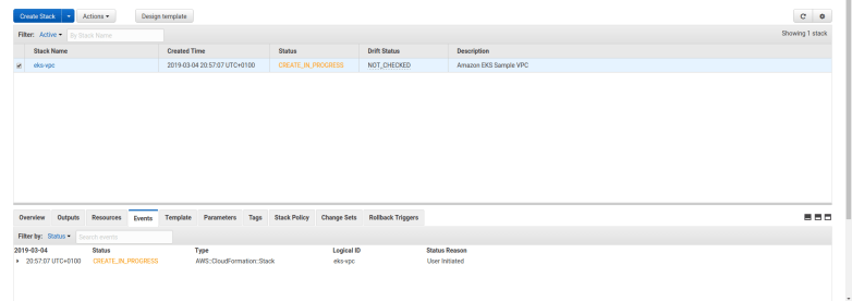
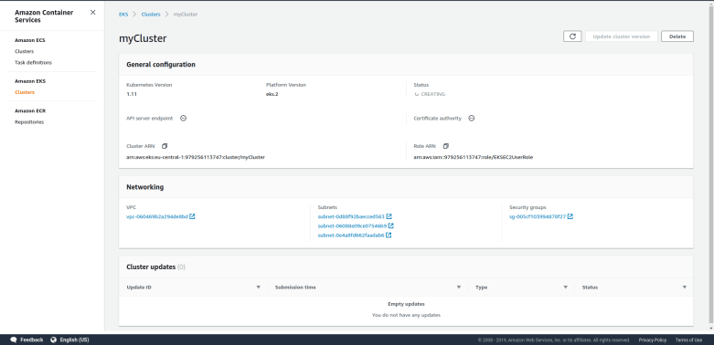
To try this out, let us assume that you have a cluster up and running and that you have submitted a deployment of two httpd instances in the cluster. To easily get to this point, you can use the scripts in my GitHub repository as follows. These scripts will also open two ssh connections, one to each of the EC2 instances which are part of the cluster (this assumes that you are using a PEM file called eksNodeKey.pem as I have done it in my examples, if not you will have to adjust the script up.sh accordingly).

# Clone repository
$ git clone https://github.com/christianb93/Kubernetes.git
$ cd Kubernetes/cluster
# Bring up cluster and two EC2 nodes
$ chmod 700 up.sh
$ ./up.sh
# Bring down nginx controller
$ kubectl delete svc ingress-nginx -n ingress-nginx
# Deploy two instances of the httpd
$ kubectl apply -f ../pods/deployment.yaml

Be patient, the creation of the cluster will take roughly 15 minutes, so time to get a cup of coffee. Note that we delete an object – the nginx ingress controller service – that my scripts generate and that we will use in a later post, but which blur the picture for today.

Now let us inspect our cluster and try out a few things. First, let us get the running pods.

$ kubectl get pods -o wide

This should give you two pods, both running an instance of the httpd. Typically, Kubernetes will distribute these two pods over two different nodes in the cluster. Each pod has an IP address called the pod IP address which is displayed in the column IP of the output. This is the IP address under which the pod is reachable from other pods in the cluster.

To verify this, let us attach to one of the pods and run curl to access the httpd running in the other pod. In my case, the first pod has IP address 192.168.232.210. We will attach to the second pod and verify that this address is reachable from there. To get a shell in the pod, we can use the kubectl exec command which executes code in a pod. The following commands extract the id of the second pod, opens a shell in this pod, installs curl and talks to the httpd in the first pod. Of course, you will have to replace the IP address of the first pod – 192.168.232.210 – with whatever your output gives you.

$ name=$(kubectl get pods --output json | \
             jq -r ".items[1].metadata.name")
$ kubectl exec -it $name "/bin/bash"
bash-4.4# apk add curl
bash-4.4# curl 192.168.232.210
<h1>It works!</h1>

Nice. So we can reach a port on pod A from any other pod in the cluster. This is what is called the flat networking model in Kubernetes. In this model, each pod has a separate IP address. All containers in the pod share this IP address and one IP namespace. Every pod IP address is reachable from any other pod in the cluster without a need to set up a gateway or NAT. Coming back to the comparison of a pod with a logical host, this corresponds to a topology where all logical hosts are connected to the same IP network.

In addition, Kubernetes assumes that every node can reach every pod as well. You can easily confirm this – if you log into the node (not the pod!) on which the second pod is running and use curl from there, directed to the IP address of the first pod, you will get the same result.

Now Kubernetes is designed to run on a variety of platforms – locally, on a bare metal cluster, on GCP, AWS or Azure and so forth. Therefore, Kubernetes itself does not implement those rules, but leaves that to the underlying platform. To make this work, Kubernetes uses an interface called CNI (container networking interface) to talk to a plugin that is responsible for executing the platform specific part of the network configuration. On EKS, the AWS CNI plugin is used. We will get into the details in a later post, but for the time being simply assume that this works (and it does).

So now we can reach every pod from every other pod. This is nice, but there is an issue – a pod is volatile. An application which is composed of several microservices needs to be prepared for the event that a pod goes down and is brought up again, be it due to a failure or simply due to the fact that an auto-scaler tries to empty a node. If, however, a pod is restarted, it will typically receive a different IP address.

Suppose, for instance, you had a REST service that you want to expose within your cluster. You use a deployment to start three pods running the REST service, but which IP address should another service in the cluster use to access it? You cannot rely on the IP address of individual pods to be stable. What we need is a stable IP address which is reachable by all pods and which routes traffic to one instance of this REST service – a bit like a cluster-internal load balancer.

Fortunately, Kubernetes services come to the rescue. A service is a Kubernetes object that has a stable IP address and is associated with a set of pods. When traffic is received which is directed to the service IP address, the service will select one of the pods (at random) and forward the traffic to it. Thus a service is a decoupling layer between the instable pod IP addresses and the rst of the cluster or the outer world. We will later see that behind the scenes, a service is not a process running somewhere, but essentially a set of smart NAT and routing rules.

This sounds a bit abstract, so let us bring up a service. As usual, a service object is described in a manifest file.

apiVersion: v1
kind: Service
metadata:
  name: alpine-service
spec:
  selector:
    app: alpine
  ports:
  - protocol: TCP
    port: 8080
    targetPort: 80

Let us call this file service.yaml (if you have cloned my repository, you already have a copy of this in the directory network). As usual, this manifest file has a header part and a specification section. The specification section contains a selector and a list of ports. Let us look at each of those in turn.

The selector plays a role similar to the selector in a deployment. It defines a set of pods that are assumed to be reachable via the service. In our case, we use the same selector as in the deployment, so that our service will send traffic to all pods brought up by this deployment.

The ports section defines the ports on which the service is listening and the ports to which traffic is routed. In our case, the service will listen for TCP traffic on port 8080, and will forward this traffic to port 80 on the associated pods (as specified by the selector). We could omit the targetPort field, in this case the target port would be equal to the port. We could also specify more than one combination of port and target port and we could use names instead of numbers for the ports – refer to the documentation for a full description of all configuration options.

Let us try this. Let us apply this manifest file and use kubectl get svc to list all known services.

$ kubectl apply -f service.yaml
$ kubectl get svc

You should now see a new service in the output, called alpine-service. Similar to a pod, this service has a cluster IP address assigned to it, and a port number (8080). In my case, this cluster IP address is 10.100.234.120. We can now again get a shell in one of the pods and try to curl that address

$ name=$(kubectl get pods --output json | \
             jq -r ".items[1].metadata.name")
$ kubectl exec -it $name "/bin/bash"
bash-4.4# apk add curl # might not be needed 
bash-4.4# curl 10.100.234.120:8080
<h1>It works!</h1>

If you are lucky and your container did not go down in the meantime, curl will already be installed and you can skip the apk add curl. So this works, we can actually reach the service from within our cluster. Note that we now have to use port 8080, as our service is listening on this port, not on port 80.

You might ask how we can get the IP address of the service in real world? Well, fortunately Kubernetes does a bit more – it adds a DNS record for the service! So within the pod, the following will work

bash-4.4# curl alpine-service:8080
<h1>It works!</h1>

So once you have the service name, you can reach the httpd from every pod within the cluster.

Connecting to services using port forwarding

Having a service which is reachable within a cluster is nice, but what options do we have to reach a cluster from the outside world? For a quick and dirty test, maybe the easiest way is using the kubectl port forwarding feature. This command allows you to forward traffic from a local port on your development machine to a port in the cluster which can be a service, but also a pod. In our case, let us forward traffic from the local port 5000 to port 8080 of our service (which is hooked up to port 80 on our pods).

$ kubectl port-forward service/alpine-service 5000:8080 

This will start an instance of kubectl which will bind to port 5000 on your local machine (127.0.0.1). You can now connect to this port, and behind the scenes, kubectl will tunnel the traffic through the Kubernetes master node into the cluster (you need to run this in a second terminal, as the kubectl process just started is still blocking your terminal).

$ curl localhost:5000
<h1>It works!</h1>

A similar forwarding can be realized using kubectl proxy, which is designed to give you access to the Kubernetes API from your local machine, but can also be used to access services.

Connect to a service using host ports

Forwarding is easy and a quick solution, but most likely not what you want to do in a production setup. What other options do we have?

One approach is to use host ports. Essentially, a host port is a port on a node that Kubernetes will wire up with the cluster IP address of a service. Assuming that you can reach the host from the outside world, you can then use the public IP address of the host to connect to a service.

To create a host port, we have to modify our manifest file slightly by adding a host port specification.

apiVersion: v1
kind: Service
metadata:
  name: alpine-service
spec:
  selector:
    app: alpine
  ports:
  - protocol: TCP
    port: 8080
    targetPort: 80
  type: NodePort

Note the additional line at the bottom of the file which instructs Kubernetes to open a node port. Assuming that this file is called nodePortService.yaml, we can again use kubectl to bring down our existing service and add the node port service.

$ kubectl delete svc alpine-service
$ kubectl apply -f nodePortService.yaml
$ kubectl get svc

We see that Kubernetes has brought up our service, but this time, we see two ports in the line describing our service. The second port (32226 in my case) is the port that Kubernetes has opened on each node. Traffic to this port will be forwarded to the service IP address and port. To try this out, you can use the following commands to get the external IP address of the first node, adapt the AWS security group such that traffic to this node is allowed from your workstation, determine the node port and curl it. If your cluster is not called myCluster, replace every occurrence of myCluster with the name of your cluster.

$ nodePort=$(kubectl get svc alpine-service --output json | jq ".spec.ports[0].nodePort")
$ IP=$(aws ec2 describe-instances --filters Name=tag-key,Values=kubernetes.io/cluster/myCluster Name=instance-state-name,Values=running --output text --query Reservations[0].Instances[0].PublicIpAddress)
$ SEC_GROUP_ID=$(aws ec2 describe-instances --filters Name=tag-key,Values=kubernetes.io/cluster/myCluster Name=instance-state-name,Values=running --output text --query Reservations[0].Instances[0].SecurityGroups[0].GroupId)
$ myIP=$(wget -q -O- https://ipecho.net/plain)
$ aws ec2 authorize-security-group-ingress --group-id $SEC_GROUP_ID --port $nodePort --protocol tcp --cidr "$myIP/32"
$ curl $IP:$nodePort
<h1>It works!</h1>

Connecting to a service using a load balancer

A node port will allow you to connect to a service using the public IP of a node. However, if you do this, this node will be a single point of failure. For a HA setup, you would typically choose a different options – load balancers.

Load balancers are not managed directly by Kubernetes. Instead, Kubernetes will ask the underlying cloud provider to create a load balancer for you which is then connected to the service – so there might be additional charges. Creating a service exposed via a load balancer is easy – just change the type field in the manifest file to LoadBalancer

apiVersion: v1
kind: Service
metadata:
  name: alpine-service
spec:
  selector:
    app: alpine
  ports:
  - protocol: TCP
    port: 8080
    targetPort: 80
  type: LoadBalancer

After applying this manifest file, it takes a few seconds for the load balancer to be created. Once this has been done, you can find the external DNS name of the load balancer (which AWS will create for you) in the column EXTERNAL-IP of the output of kubectl get svc. Let us extract this name and curl it. This time, we use the jsonpath option of the kubectl command instead of jq.

$ host=$(kubectl get svc alpine-service --output  \
         jsonpath="{.status.loadBalancer.ingress[0].hostname}")
$ curl $host:8080
<h1>It works!</h1>

If you get a “couldn not resolve hostname” error, it might be that the DNS entry has not yet propagated through the infrastructure, this might take a few minutes.

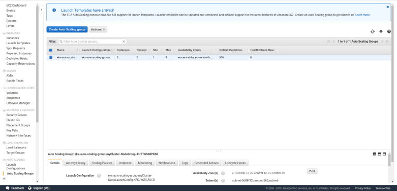
What has happened? Behind the scenes, AWS has created an elastic load balancer (ELB) for you. Let us describe this load balancer.

$ aws elb describe-load-balancers --output json
{
    "LoadBalancerDescriptions": [
        {
            "Policies": {
                "OtherPolicies": [],
                "LBCookieStickinessPolicies": [],
                "AppCookieStickinessPolicies": []
            },
            "AvailabilityZones": [
                "eu-central-1a",
                "eu-central-1c",
                "eu-central-1b"
            ],
            "CanonicalHostedZoneName": "ad76890d448a411e99b2e06fc74c8c6e-2099085292.eu-central-1.elb.amazonaws.com",
            "Subnets": [
                "subnet-06088e09ce07546b9",
                "subnet-0d88f92baecced563",
                "subnet-0e4a8fd662faadab6"
            ],
            "CreatedTime": "2019-03-17T11:07:41.580Z",
            "SecurityGroups": [
                "sg-055b253a63c7aba0a"
            ],
            "Scheme": "internet-facing",
            "VPCId": "vpc-060469b2a294de8bd",
            "LoadBalancerName": "ad76890d448a411e99b2e06fc74c8c6e",
            "HealthCheck": {
                "UnhealthyThreshold": 6,
                "Interval": 10,
                "Target": "TCP:30829",
                "HealthyThreshold": 2,
                "Timeout": 5
            },
            "BackendServerDescriptions": [],
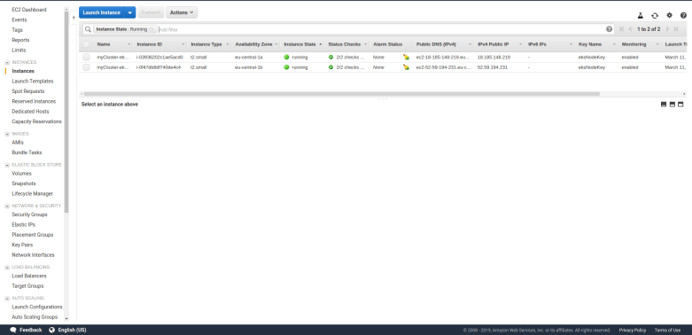
            "Instances": [
                {
                    "InstanceId": "i-0cf7439fd8eb65858"
                },
                {
                    "InstanceId": "i-0fda48856428b9a24"
                }
            ],
            "SourceSecurityGroup": {
                "GroupName": "k8s-elb-ad76890d448a411e99b2e06fc74c8c6e",
                "OwnerAlias": "979256113747"
            },
            "DNSName": "ad76890d448a411e99b2e06fc74c8c6e-2099085292.eu-central-1.elb.amazonaws.com",
            "ListenerDescriptions": [
                {
                    "PolicyNames": [],
                    "Listener": {
                        "InstancePort": 30829,
                        "LoadBalancerPort": 8080,
                        "Protocol": "TCP",
                        "InstanceProtocol": "TCP"
                    }
                }
            ],
            "CanonicalHostedZoneNameID": "Z215JYRZR1TBD5"
        }
    ]
}

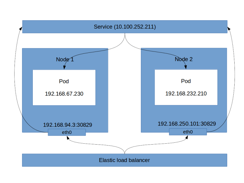
This is a long output, let us see what this tells us. First, there is a list of instances, which are the instances of the nodes in your cluster. Then, there is the block ListenerDescriptions. This block specificies, among other things, the load balancer port (8080 in our case, this is the port that the load balancer exposes) and the instance port (30829). You will note that these are also the ports that kubectl get svc will give you. So the load balancer will send incoming traffic on port 8080 to port 30829 of one of the instances. This in turn is a host port as discussed before, and therefore will be connected to our service. Thus, even though technically not fully correct, the following picture emerges (technically, a service is not a process, but a collection of iptables rules on each node, which we will look at in more detail in a later post).

LoadBalancerService

Using load balancers, however, has a couple of disadvantages, the most obvious one being that each load balancer comes with a cost. If you have an application that exposes tens or even hundreds of services, you clearly do not want to fire up a load balancer for each of them. This is where an ingress comes into play, which can distribute incoming HTTP(S) traffic across various services and which we will study in one of the next posts.

There is one important point when working with load balancer services – do not forget to delete the service when you are done! Otherwise, the load balancer will continue to run and create charges, even if it is not used. So delete all services before shutting down your cluster and if in doubt, use aws elb describe-load-balancers to check for orphaned load balancers.

Creating services in Python

Let us close this post by looking into how services can be provisioned in Python. First, we need to create a service object and populate its metadata. This is done using the following code snippet.

service = client.V1Service()
service.api_version = "v1"
service.kind = "Service"
metadata = client.V1ObjectMeta(name="alpine-service")
service.metadata = metadata
service.type="LoadBalancer"

Now we assemble the service specification and attach it to the service object.

spec = client.V1ServiceSpec()
selector = {"app": "alpine"}
spec.selector = selector
spec.type="LoadBalancer"
port = client.V1ServicePort(
              port = 8080, 
              protocol = "TCP", 
              target_port = 80 )
spec.ports = [port]
service.spec = spec

Finally, we authenticate, create an API endpoint and submit the creation request.

config.load_kube_config()
api = client.CoreV1Api()
api.create_namespaced_service(
         namespace="default", 
         body=service)

If you have cloned my GitHub repository, you will find a script network/create_service.py that contains the full code for this and that you can run to try this out (do not forget to delete the existing service before running this).

Single qubit NMR based quantum computation

In the previous post, we have sketched the basic ideas behind NMR based quantum computation. In this post, we will discuss single qubits and single qubit operations in more depth.

The rotating frame of reference

In NMR based quantum computing, quantum gates are realized by applying oscillating magnetic fields to our probe. As an oscillating field is time dependent, the Hamiltonian will be time dependent as well, making some calculations a bit more difficult. To avoid this, it is useful to pass to a different frame of reference, called the rotating frame of reference.

To explain this, let us first study a more general setting. Assume that we are looking at a quantum system with Hamiltonian H and a state vector |\psi \rangle. Suppose further that we are given a unitary group, i.e. a time-dependent unitary operator

T(t) = e^{-iAt}

with a hermitian matrix A. We can then consider the transformed vector

|\tilde{\psi}\rangle = T(t) |\psi \rangle

Using the product rule and the Schrödinger equation, we can easily calculate the time derivative of this vector and obtain

i \hbar \frac{d}{dt} |\tilde{\psi}\rangle = \hbar A |\tilde{\psi} \rangle + T(t) H |\psi\rangle = \tilde{H} |\tilde{\psi}\rangle

with

\tilde{H} = THT^* + \hbar A

In other words, the transformed vector again evolves over time according to an equation which is formally a Schrödinger equation if we replace the original Hamiltonian by the transformed Hamiltonian \tilde{H}.

Let us now apply this to the system describing a single nuclear spin with spin 1/2 in a constant magnetic field B along the z-axis of the laboratory system. In the laboratory frame, the Hamiltonian is then given by

H = \omega I_z

with the Larmor frequency \omega and the spin operator

I_z = \frac{\hbar}{2} \sigma_z

We now pass into a new frame of reference by applying the transformation

T(t) = \exp ( \frac{i\omega_{ref}}{\hbar} t I_z )

with an arbitratily chosen reference frequency \omega_{ref}
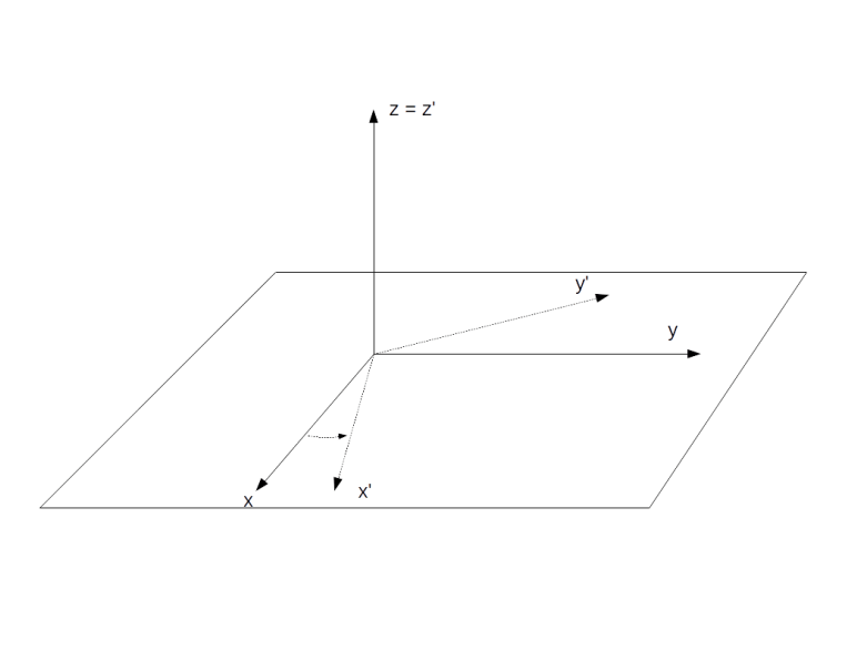
. Geometrically, this is a rotation around the z-axis by the angle \omega_{ref}t. Using the formula above and the fact that T commutes with the original Hamiltonian, we find that the transformed Hamiltonian is

\tilde{H} = (\omega - \omega_{ref}) I_z

This is of the same form as the original Hamiltonian, with a corrected Larmor frequency

\Omega = \omega - \omega_{ref}

In particular, the Hamiltonian is trivial if the reference frequency is equal to the Larmor frequency.

Intuitively, this is easy to understand. We know that the time evolution in the laboratory frame is described by a precession with the frequency \omega. When we choose \omega_{ref} = \omega
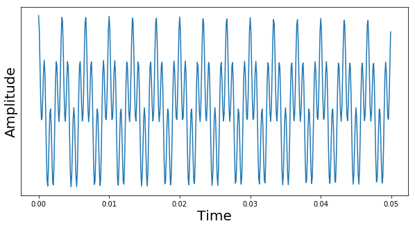
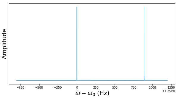
, we place ourselves in a frame of reference rotating with the same frequency around the z-axis. In this rotating frame, the state vector will be constant, corresponding to the fact that the new Hamiltonian vanishes. If we choose a reference frequency different from the Larmor frequency, we will observe a precession with the frequency \Omega.

RotatingFrame

Let us now repeat this for a different Hamiltonian – the Hamiltonian that governs the time evolution in the presence of an oscillating magnetic field. More precisely, we will look at the Hamiltonian of a rotating magnetic field (which is a good approximation for an oscillating magnetic field by an argument known as rotating wave approximation, see my notes for more details on this). In the presence of such a field, the Hamiltonian in the laboratory frame is

H = \omega I_z + \omega_{nut} [I_x \cos (\omega_{ref}t + \Phi_p) + I_y \sin (\omega_{ref}t + \Phi_p) ]

To calculate the Hamiltonian in the rotating frame, we have – according to the above formula – to apply the conjugation with T to each of the terms appearing in this Hamiltonian and add a correction term.

Now the transformation T is a rotation around the z-axis, and the result of applying a rotation around the z-axis to the operators Ix and Iy is well known and in fact easy to calculate using the commutation relations between the Pauli matrices. The correction term cancels the first term of the Hamiltonian as above. The transformed Hamiltonian is then given by

\tilde{H} = \omega_{nut} [I_x \cos \Phi_p + I_y \sin \Phi_p ]

In other words, the time dependence has disappeared and only the phase term remains. Again, this is not really surprising – if we look at a rotating magnetic field from a frame of reference that is rotating around the same axis with the same frequency, the result is a constant magnetic field.

The density matrix of a single qubit

We are now ready to formally describe a single qubit, given by all nuclei at a specific position in a system consisting of a large number of molecules. According to the formalism of statistical quantum mechanics, this ensemble is described by a 2×2 density matrix \rho. The time evolution of this density matrix is governed by the Liouville-von Neumann equation

i\hbar \frac{d}{dt} \rho = [H,\rho]

The density matrix is a hermitian matrix with trace 1. Therefore the matrix \rho - \frac{1}{2} is a traceless hermitian matrix. Any such matrix can be expressed as a linear combination of the Pauli matrices with real coefficients. Consequently, we can write

\rho(t) = \frac{1}{2} + f(t) \cdot I

where f is a three-vector with real coefficients and the dot product is a shorthand notation for

f \cdot I = f_x I_x + f_y I_y + f_z I_z

Similarly, the most general time-independent Hamiltonian can be written as

H = \frac{1}{2} tr(H) + a \cdot I

We can remove the trace by adding a constant, which does not change the physics and corresponds to a shift of the energy scale. Further, we can express the vector a as the product of a unit vector and a scalar. Thus the most general Hamiltonian we need to consider is

H = \omega_{eff} n \cdot I

with a real number \omega_{eff} (the reason for this notation will become apparent in a second) and a unit vector n.

Let us now plug this into the Liouville equation. Applying the very useful general identity (which is easily proved by a direct calculation)

[a\cdot I, b \cdot I] = i \hbar (a \times b) \cdot I

for any two vectors a and b, we find that

\dot{f} = - \omega_{eff} [f \times n]

This equation is often called the Bloch equation. By splitting f into a component perpendicular to n and a component parallel to n, one can easily see that the solution is a rotation around the axis n with frequency \omega_{eff}.

What is the physical interpretation of this result and the physical meaning of f? To see this, let us calculate the expectation value of the magnetic moment induced by the spin of our system. The x-component of the magnetic moment, for instance, corresponds to the observable \gamma I_x. Therefore, according to the density matrix formalism, the expectation value of the x-component of the magnetic moment \mu is

\langle \mu_x \rangle = \gamma tr (\rho I_x)

If we compute the matrix product \rho I_x and use the fact that the trace of a product of two different Pauli matrices is zero, we find that the only term that contributes to the trace is the term fx, i.e.

\langle \mu_x \rangle = \frac{\gamma \hbar^2}{4} f_x

Similar calculations work for the other components and we find that, up to a constant, the vector f is the net magnetic moment of the probe.

A typical NMR experiment

After all these preparations, we now have all tools at our disposal to model the course of events during a typical NMR experiment in terms of the density matrix.

Let us first try to understand the initial state of the system. In a real world experiment, none of the qubits is fully isolated. In addition, the qubits interact, and they interact with the surroundings. We can model these interactions by treating the qubits as being in contact with a heat bath of constant temperature T. According to the rules of quantum statistical mechanics, the equilibrium state, i.e. the state into which the system settles down after some time, is given by the Boltzmann distribution, i.e.

\rho(t=0) = \frac{1}{Z} \exp (- \frac{H}{kT})

In the absence of an additional rotating field, the Hamiltonian in the laboratory frame is given by

H = \omega I_z

Therefore

\rho(t=0) = \frac{1}{Z} \exp ( \frac{-\omega}{kT} I_z)

Using the relations

I_z = \frac{\hbar}{2} \sigma_z

and

\omega = -\gamma B \sigma_z

with the gyromagnetic moment \gamma
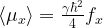
, we can write this as

\rho(t=0) = \frac{1}{Z} \exp ( \frac{1}{2} {{\hbar \gamma B}\over{kT}} \sigma_z)

Let us now introduce the energy ratio

\beta = \frac{\hbar \gamma B}{kT}

The energy in the numerator is the energy scale associated with the Larmor frequency. For a proton in a magnetic field of a few Tesla, for example, this will be in the order of 10-25 Joule. The energy in the denominator is the thermal energy. If the experiment is conducted at room temperature, say T=300K, then this energy is in the order of 10-21 Joule (see this notebook for some calculations). This yields a value of roughly 10-4 for \beta. If we calculate the exponential in the Boltzmann distribution by expanding into a power series, we can therefore neglect all terms except the constant term and the term linear in \beta. This gives the approximation

\rho(t=0) = \frac{1}{Z} (1 + \frac{1}{2} \beta \sigma_z)

called the high temperature approximation. We can determine the value of Z by calculating the trace and find that Z = 2, so that

\rho(t=0) = \frac{1}{2} + \frac{1}{4} \beta \sigma_z = \begin{pmatrix} \frac{1}{2} + \frac{\beta}{4} & 0 \\ 0 & \frac{1}{2} - \frac{\beta}{4} \end{pmatrix} = \frac{1}{2} + \frac{1}{2} \frac{\beta}{\hbar} I_z

If we compare this to the general form of the density matrix discussed above, we find that the thermal state has a net magnetization in the direction of the z-axis (for positive \beta). This is what we expect – with our sign conventions, the energy is lowest if the spin axis is in the direction of the z-axis, so that slightly more nuclei will have their spins oriented in this direction, leading to a net magnetic moment.

To calculate how this state changes over time, we again pass to the rotating frame of reference. As the initial density matrix clearly commutes with the rotation around the z-axis, the density matrix in the rotating frame is the same. If we choose the reference frequency to be exactly the Larmor frequency, the Hamiltonian given by the static magnetic field along the z-axis vanishes, and the density matrix does not change over time.

When, however, we apply an additional pulse, i.e. an additional rotating magnetic field, for some time \tau
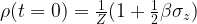
, this changes. We have already seen that in the rotating frame, this pulse adds an additional term

\omega_{nut} (I_x \cos \Phi_p + I_y \sin \Phi_p)

to the Hamiltonian. This has the form discussed above – a scalar times a dot product of a unit vector with the vector I = (Ix, Iy, Iz). Therefore, we find that the time evolution induced by this Hamiltonian is a rotation around the vector

(\cos \Phi_p, \sin \Phi_p, 0)

with the frequency \omega_{nut}
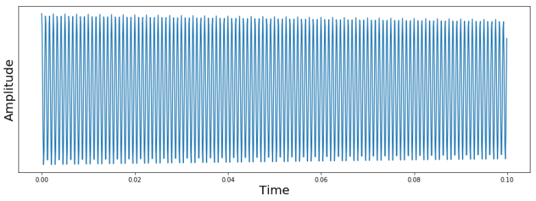
. If, for instance, we choose \Phi_p = 0, the vector f – and thus the magnetic moment – will slowly rotate around the x-axis. If we turn off the pulse after a time \tau such that

\omega_{nut} \tau = \frac{\pi}{2}

the net magnetization will be parallel to the y-axis. After the pulse has been turned off, the density matrix in the rotating frame is again constant, so the magnetic moment stays along the y-axis. In the laboratory frame, however, this corresponds to a magnetic moment which rotates with the Larmor frequency around the z-axis. This magnetic moment will induce a voltage in a coil placed in the x-y-plane which can be measured. The result will be an oscillating current, with frequency equal to the Larmor frequency. Over time, the state will slowly return into the thermal equilibrium, resulting in a decay of the oscillation.

This is a good point in time to visualize what is happening. Given the explicit formulas for the density matrix derived above, it is not difficult to numerically simulate the state changes and NMR signals during an experiment as the one that we have just described (if you want to take a look at the required code, you can find a Python notebook here)

The diagram below shows the result of such a simulation. Here, we have simulated a carbon nucleus in a TCE (Trichloroethylene) molecule. This molecule – pictured below (source Wikipedia) – has two central carbon nuclei.

Trikloreten.svg

A small percentage of all TCE molecules in a probe will have two 13C nuclei instead of the more common 12C nuclei, which have spin 1/2 and therefore should be visible in the NMR spectrum. At 11.74 Tesla, an isolated 13C carbon nucleus has a Larmor precession frequency of 125 MHz. However, when the nuclei are part of a larger molecule as in our case, each nucleus is shielded from an external magnetic field by the surrounding cloud of electrons. As the electron configuration for both nuclei is different, the observed Larmor frequencies differ by a small amount known as the chemical shift.

At the start of the simulation, the system was put into a thermal state. Then, an RF pulse was applied to flip the magnetization in the direction of the x-axis, and then a sample was taken over 0.1 seconds, resulting in the following signal.

SingleNucleusNMRSignal

The signal that we see looks at the first glance as expected. We see an oscillating signal with an amplitude that is slowly decaying. However, you might notice that the frequency of the oscillation is clearly not 125 MHz. Instead, the period is roughly 0.001 seconds, corresponding to a frequency of 1200 Hz. The reason for this is that in an NMR spectrometer, the circuit processing the received signal will typically apply a combination of a mixer and a low pass filter to effectively shift the frequency by an adjustable reference frequency. In our case, the reference frequency was adjusted to be 1200 Hz above the Larmor frequency of the carbon nucleus, so the signal will oscillate with a frequency of 1200 Hz. In practice, the reference frequency determines a window in the frequency space in which we can detect signals, and all frequencies outside this window will be suppressed by the low pass filter.

Now let us take a look at a more complicated signal. We again place the system in the thermal equilibrium state first, but then apply RF pulses to flip the spin of both carbon nuclei into the x-axis (in a simulation, this is easy, in a real experiment, this requires some thought, as the Larmor frequencies of these two carbon nuclei differ only by a small chemical shift of 900 Hz). We then again take a sample and plot the signal. The result is shown below.

TwoNucleiNMRSignal

This time, we see a superposition of two oscillations. The first oscillations is what we have already seen – an oscillation with 1200 Hz, which is the difference of the chosen reference frequency and the Larmor frequency of the first carbon. The second oscillation corresponds to a frequency of roughly 300 Hz. This is the signal caused by the Larmor precession of the second spin. As we again measure the difference between the real frequency and the reference frequency, we can conclude that this frequency differs from the Larmor frequency of the first spin by 900 Hz.

In reality, the signal that we observe is the superposition of many different oscillations and is not easy to interpret – even with a few oscillations, it soon becomes impossible to extract the frequencies by a graphical analysis as we have done it so far. Instead, one usually digitizes the signal and applies a Fourier transform (or, more precisely, a discrete Fourier transform). The following diagram shows the result of applying such a DFT to the signal above.

TwoNucleiNMRSignalFFT

Here, we have shifted the x-axis by the difference between the Larmor frequency \omega_0 of the first nucleus and the reference frequency, so that the value zero corresponds to \omega_0. We clearly see two peaks. The first peak at zero, i.e. at Larmor frequency \omega_0, is the signal emitted by the first nucleus. The second peak is shifted by 900 Hz and is emitted by the second nucleus. In general, each nucleus will result in one peak (ignoring couplings that we will study in a later post) and the differences between the peaks belonging to nuclei of the same isotope are the chemical shifts.

Let us quickly summarize what we have learned. An ensemble of spin systems is described by a density which in turn is given by the net magnetization vector f. The result of applying a pulse to this state is a rotation around an axis given by the phase of the pulse (in fact, the phase can be adjusted to rotate around any axis in the x-y-plane, and as any rotation can be written as a decomposition of such rotations, we can generate an arbitrary rotation). The net magnetization can be measured by placing a coil close to the probe and measuring the induced voltage.

This does already look like we are able to produce a reasonable single qubit. The vector f appears to correspond – after some suitable normalization – to points on the Bloch sphere, and as we can realize rotations, we should be able to realize arbitrary single qubit quantum gates. But what about multiple qubits? Of course a molecule typically has more than one nucleus, and we could try to use additional nuclei to create additional qubits, but there is a problem – in order to realize multi-qubit gates, these qubits have to interact. In addition, we need to be able to prepare our NMR system in a useful initial state and, at the end of the computation, we need to measure the outcome. These main ingredients of NMR based quantum computing will be the subject of the next post.

Kubernetes 101 – creating pods and deployments

In the last posts, we have seen how we can set up a Kubernetes cluster on Amazons EKS platform and spin up our first nodes. Today, we will create our first workloads and see pods and deployments in action.

Creating pods

We have already introduces pods in an earlier post as the smallest units that Kubernetes manages. To create pods, there are several options. First, we can use the kubectl command line tool and simply pass the description of the pod as arguments. Second, we can use a so-called manifest file which contains the specification of the pod, which has the obvious advantage that this file can be reused, put under version control, developed and tested, according to the ideas of the “Infrastructure as a code” approach. A manifest file can either be provided in JSON format or using the YAML markup language. And of course, we can again use the Kubernetes API directly, for instance by programming against the Python API.

In this post, we will demonstrate how to create pods using manifest file in YAML format and Python scripts. We start with a YAML file which looks as follows.

apiVersion: v1
kind: Pod
metadata:
  name: naked-pod-demo
  namespace: default
spec:
  containers:
  - name: naked-pod-demo-ctr
    image: nginx

Let us go through this file step by step to understand what it means. First, this is a YAML file, and YAML is essentially a format for specifying key-value pairs. Our first key is apiVersion, with value v1. This is the first line in all manifest files and simply specifies the API version that we will use.

The next key – kind – specifies the type of Kubernetes resource that we want to access, in this case a pod. The next key is metadata. The value of this key is a dictionary that again has two keys – name and namespace. The name is the name that our pod will have. The namespace key specifies the namespace in which the pod will start (namespaces are a way to segment Kubernetes resources and are a topic for a future post, for the time being we will simply use the so-called default namespace).

The next key – spec now contains the actual specification of the pod. This is where we tell Kubernetes what our pod should be running. Remember that a pod can contain one or more application containers. Therefore there is a key containers, which, as a value, has a list of containers. Each container has a name and further attributes.

In our case, we create one container and specify that the image should be nginx. At this point, we can specify every image that we could also specify if we did a docker run locally. In this case, Kubernetes will pull the nginx image from the default docker registry and run it.

So let us now trigger the creation of a pod by passing this specification to kubectl. To do this, we use the following command (assuming that you have saved the file as naked_pod.yaml, the reason for this naming will become clear later).

kubectl apply -f naked_pod.yaml

After a few seconds, Kubernetes should have had enough time to start up the container, so let us use kubectl to check whether the node has been created.

$ kubectl get pods 
NAME             READY   STATUS    RESTARTS   AGE
naked-pod-demo   1/1     Running   0          38s

Nice. Let us take a closer look at this pod. If you run kubectl get pods -o wide, kubectl will give you a bit more information on the pod, including the name of the node on which the pod is running. So let us SSH into this node. To easily log into one of your nodes (the first node in this case, change Node to 1 to log into the second node), you can use the following sequence of commands. This will open the SSH port for all instances in the cluster for incoming connections from the your current IP address. Note that we use the cluster name as a filter, so you might need to replace myCluster in the commands below by the name of your cluster.

$ Node=0
$ IP=$(aws ec2 describe-instances --output text --filters Name=tag-key,Values=kubernetes.io/cluster/myCluster Name=instance-state-name,Values=running --query Reservations[$Node].Instances[0].PublicIpAddress)
$ SEC_GROUP_ID=$(aws ec2 describe-instances  --output text --filters Name=tag-key,Values=kubernetes.io/cluster/myCluster Name=instance-state-name,Values=running --query Reservations[0].Instances[0].SecurityGroups[0].GroupId)
$ myIP=$(wget -q -O- https://ipecho.net/plain)
$ aws ec2 authorize-security-group-ingress --group-id $SEC_GROUP_ID --port 22 --protocol tcp --cidr $myIP/32
$ ssh -i ~/eksNodeKey.pem ec2-user@$IP

Use this – or your favorite method (if you use my script up.sh to start the cluster, it will already open ssh connections to both nodes for you) – to log into the node on which the pod has been scheduled by Kubernetes and execute a docker ps there. You should see that, among some management containers that Kubernetes brings up, a container running nginx appears.

Now let us try a few things. First, apply the YAML file once more. This will not bring up a second pod. Instead, Kubernetes realizes that a pod with this name is already running and tells you that no change has been applied. This makes sense – in general, a manifest file specifies a target state, and we are already in the target state, so there is no need for action.

Now, on the EKS worker node on which the pod is running, use docker kill to actually stop the container. Then wait for a few seconds and do a docker ps again. Surprisingly, you will see the container again, but with a different container ID. What happened?

The answer is hidden in the logfiles of the component of Kubernetes that controls a single node – the kubelet. On the node, the kubelet is started using systemctl (you might want to verify this in the AWS provided bootstrap.sh script). So to access its logs, we need

$ journalctl -u kubelet

Close to the end of the logfile, you should see a line stating that … container … is dead, but RestartPolicy says that we should restart it. In fact, the kubelet constantly monitors the running containers and looks for deviations from the target state. The restart policy is a piece of the specification of a pod that tells the kubelet how to handle the case that a container has died. This might be perfectly fine (for batch jobs), but the default restart policy is Always, so the the kubelet will restart our container.

This is nice, but now let us simulate a more drastic event – the node dies. So on the AWS console, locate the node on which the pod is running and terminate the pod.

After a few seconds, you will see that a new node is created, thanks to the AWS auto-scaling group that controls our nodes. However, if you check the status of the pods using kubectl get pods, you will see that Kubernetes did not reschedule the pod on a different node, nor does it restart the pod once the replacement node is up and running again. So Kubernetes takes care (via the kubelet) of the containers that belong to a pod on a per-node level, but not on a per-cluster level.

In productions, this is of course typically not what you want – instead, it would be nice if Kubernetes could monitor the pods for you and restart them automatically in case of failure. This is what a deployment does.

Replica sets and deployments

A deployment is an example for a more general concept in Kubernetes – controllers. Basically, this is a component that constantly monitors the cluster state and makes changes if needed to get back into the target state. One thing that a deployment does is to automatically bring up a certain number of instances called replicas of a Docker image and distribute the resulting pods across the cluster. Once the pods are running, the deployment controller will monitor them and take action of the number of pods running deviates from the desired number of pods. As an example, let us consider the following manifest file.

apiVersion: apps/v1
kind: Deployment
metadata:
  name: alpine
spec:
  selector:
    matchLabels:
      app: alpine
  replicas: 2
  template:
    metadata:
      labels:
        app: alpine
    spec:
      containers:
        - name: alpine-ctr
          image: httpd:alpine

The first line is specifying the API version as usual (though we need to use a different value for the API version, the additional apps is due to the fact that the Deployment API is part of the API group apps). The second line designates the object that we want to create as a deployment. We then again have a name which is part of the metadata, followed by the actual specification of the deployment.

The first part of this specification is the selector. To understands its role, recall that a deployment is supposed to make sure that a specified number of pods of a given type are running. Now, the term “of a given type” has to be made precise, and this is what the selector is being used for. All pods which are created by our deployment will have a label with key “app” and value “alpine”. The selector field specifies that all pods with that label are to be considered as pods controlled by the deployment, and our controller will make sure that there are always exactly two pods with this label.

The second part of the specification is the template that the deployment uses to create the pods controlled by this deployment. This looks very much like the definition of a pod as we have seen it earlier. However, the label that is specified here of course needs to match the label in the selector field (kubectl will actually warn you if this is not the case).

Let us now delete our existing pod, run this deployment and see what is happening. Save the manifest file as deployment.yaml, apply it and then list the running nodes.

$ kubectl delete -f naked_pod.yaml
$ kubectl apply -f deployment.yaml
deployment.apps/alpine created
$ kubectl get pods
NAME                      READY   STATUS    RESTARTS   AGE
alpine-8469fc798f-rq92t   1/1     Running   0          21s
alpine-8469fc798f-wmsqc   1/1     Running   0          21s

So two pods have been created and scheduled to nodes of our cluster. To inspect the container further, let us ask kubectl to provide all details as JSON and use the wonderful jq to process the output and extract the container information from it (you might need to install jq to run this).

$ kubectl get pods --output json | jq ".items[0].spec.containers[0].image"
"httpd:alpine"

So we see that the pods and the containers have been created according to our specification and run the httpd:alpine docker image.

Let us now repeat our experiment from before and stop one of the node. To do this, we first extract the instance ID of the first instance using the AWS CLI and then use the AWS CLI once more to stop this instances.

$ instanceId=$(aws ec2 describe-instances --output text --filters Name=tag-key,Values=kubernetes.io/cluster/myCluster Name=instance-state-name,Values=running --query Reservations[0].Instances[0].InstanceId)
$ aws ec2 terminate-instances --instance-ids $instanceId

After some time, Kubernetes will find that the instance has died, and if you run a kubectl get nodes, you will find that the node has disappeared. If you now run kubectl get nodes -o wide, however, you will still find two pods, but now both are running on the remaining node. So the deployment controller has replaced the pod that went down with our node by a new pod on the remaining node. This behaviour is in fact not realized by the deployment, but by the underlying ReplicaSet. We could also create a replica set directly, but a deployment offers some additional features, like the possibility to run a rolling upgrade automatically.

Creating deployments in Python

Having discussed how to create a deployment from a YAML file, let us again do the same thing in Python. The easiest approach is to walk our way upwards through the YAML file. After the usual preparations (imports, loading the configuration), we therefore start with the specification of the container.

import client
container = client.V1Container(
              name="alpine-ctr",
              image="httpd:alpine")

This is similar to our YAML file – in each pod, we want to run a container with the httpd:alpine image. Having the container object, we can now create the template section.

template = client.V1PodTemplateSpec(
        metadata=client.V1ObjectMeta(
                   labels={"app": "alpine"}),
        spec=client.V1PodSpec(containers=[container]))

Again, note the label that we will use later to select the pods that our deployment controller is supposed to watch. Now we put the template into the specification part of our controller.

selector = client.V1LabelSelector(
              match_labels={"app" : "alpine"})
spec = client.V1DeploymentSpec(
        replicas=2,
        template=template, 
        selector=selector)

And finally, we can create the actual deployment object and ask Kubernetes to apply it – the complete Python script is available for download here).

deployment = client.V1Deployment(
       api_version="apps/v1",
       kind="Deployment",
       metadata=client.V1ObjectMeta(name="alpine"),
       spec=spec)

apps.create_namespaced_deployment(
              namespace="default", body=deployment)

This completes our post for today. We now know how to create pods and deployments to run Docker images in our cluster. In the next few posts, we will look at networking in Kubernetes – services, load balancers, ingress and all that.

Bulk quantum computing with nuclear spin systems

The theoretical foundations of universal quantum computing were essentially developed in the nineties of the last century, when the first native quantum algorithms and quantum error correction were discovered. Since then, physicists and computer scientists have been working on physical implementations of quantum computing. One of the first options that moved into the focus was to use a technology known as nuclear magnetic resonance (NMR) to develop universal quantum computers. In this post, we give a brief overview of NMR based quantum computing and prepare to dive into some advanced topics in the next few posts.

Introduction to NMR

Nuclear magnetic resonance is not a new technology. It was already developed to a high degree when quantum computation was initially discussed, and was therefore a natural choice for first implementations.

So what is NMR? Recall that all matter (as we know it) consists of molecules which, in turn, are compounds of atoms. Each atom consists of a nucleus and a cloud of electrons.

A nucleus is itself not an elementary particle, but is a composite system, formed by protons and neutrons (which again are not elementary but consist of quarks). As every elementary particle, each constituent of a nucleus has a spin degree of freedom. These spins add up to a total spin. Of course, the spin depends on the quantum mechanical state of the nucleus, but typically, the energy gap between the ground state and the first excited state is so high that at room temperature, it is a good approximation to assume that the spin of the nucleus is the ground state spin. The value of this spin of course depends on the structure of the nucleus. Some nuclei, like deuterium, have spin one, some – like 12C have spin zero, some like 13C have spin 1/2, and some have higher spins.

Of course the nuclear spin interacts with an external magnetic field. The strength of this interaction is determined by the coupling between the magnetic field and the spin which is expressed by the gyromagnetic moment of the nucleus.

Now suppose we are given a probe of a substance with nuclear spin 1/2 that is subject to an external field along some axis, say the z-axis. Let us simplify the discussion a bit by looking at a single nucleus only and ignoring all spatial degrees of freedom. The nuclear spin is then described by a two-level system, i.e. a qubit. The Hamiltonian of this system is

H = - \frac{\hbar}{2} \gamma B \sigma_z

where \gamma is the gyromagnetic moment, B is the magnetic field in the z-direction and \sigma_z is the usual Pauli Z-operator, i.e. the Hamiltonian is simply a multiple of the Pauli Z operator. Consequently, the time evolution operator is

U(t) = \exp \left( - \frac{i}{\hbar} H t \right) = \exp \left( - \omega i \frac{\hbar}{2} \sigma_z \right)

with \omega = - \gamma B. Thus, on the Bloch sphere, the time evolution is a rotation around the z-axis with frequency \omega. This rotation is called the Larmor precession and the frequency is called the Larmor frequency. For typical nuclei and fields, the Larmor frequency is in the order of a few hundred MHz.

Let us now suppose that the spin is originally in the ground state, i.e. pointing to the north pole of the Bloch sphere.

BlochSphereGroundState

What happens if we now apply an external additional magnetic pulse? The answer will obviously depend on the frequency and direction of the pulse. A detailed analysis that we will carry out in a later post shows that if the frequency of the pulse is equal to the Larmor frequency, the effective Hamiltonian during the pulse (in a rotating frame of reference) is proportional to the Pauli X matrix. Therefore the time evolution operator during the pulse corresponds to a rotation around the X-axis. If we time the pulse correctly so that the angle of this rotation is \frac{\pi}{2}
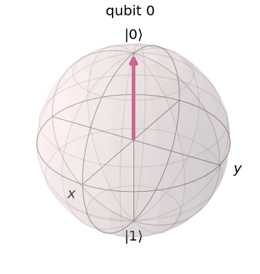
, then the nuclear spin will flip into a direction perpendicular to the z-axis.

BlochSphereRotateAroundX

After the pulse has completed, the time evolution is now again given by the rotation around the z-axis with the Larmor frequency. Consequently, the spin axis will start to precess around the z-axis. This spin precession represents a rotating magnetic moment and creates an oscillating magnetic field which in turn can be detected by placing a coil close the probe so that the rotating field will induce a voltage in the coil. Of course, the frequency of the observed signal will be that of the rotation, i.e. the Larmor frequency of the nucleus in question. We therefore find that we obtain a resonance peak at the Larmor frequency if we slowly vary the frequency of the external pulse.

In a probe that contains several different types of nuclei, we will observe more than one resonance peak – one at the Larmor frequency of each of the involved nuclei. The location and relative strength of these peaks can be used to determine the nuclei that make up the probe, and can even yield insights into the interactions between the nuclei and therefore the structure of the molecule. This technique is called nuclear magnetic resonance (NMR).

How NMR can be used for quantum computation

This description of the NMR process is on a very heuristic level, but it can be made precise (and we will look at a few more details in the next few posts). But let us take this for granted for today and let us discuss how this technology can be applied to implement a universal quantum computer.

At the first glance, this looks like a perfect match. If we pick a nucleus like 13C which has spin 1/2, the spin degree of freedom is described by a two-level system which makes for a perfect qubit. We have already indicated above that rotations on the Bloch sphere, i.e. one-qubit operations, can be realized by applying correctly timed magnetic fields. Given that the NMR technology is already highly developed, it appears that NMR should be a good candidate for an implementation.

However, there are few subtleties that we have ignored. First, we have not yet discussed multi-qubit systems. Of course, in a typical molecule, there is more than one nucleus. Not all nuclei have spin 1/2, but for some molecules, we will find several spin 1/2 nuclei which could serve as qubits. In one of the first applications of NMR to quantum computing (see [3]) for instance, a custom designed molecule was chosen to represent five qubits. Of course, this method is difficult to scale if we want to build systems with more than 20 or 50 qubits, but for a low number of qubits, it has been demonstrated to work.

Another problem which we have largely ignored so far is that of course, the probe that we use consists of a very large number of molecules. When we place this probe in our external magnetic field, the spin axis of the individual nuclei will not point all in the same direction, but instead we expect a random pattern of spin orientations. How can we then prepare the system in a well defined initial state? And how can we avoid that the individual signals created by each qubit cancel each other completely because of the random orientation of the spin axis? Of course we could try to cool down the system to a very low temperature to force all spin nuclei into the ground state, but this would make dealing with the system difficult and take very long. A solution to this problem was presented in [4] and [5] – it turns out that even though it appears almost impossible to prepare the system in a pure state, one can prepare it in a state which has properties similar to a pure state and is sufficient to do quantum computation.

In fact, the NMR technology quickly turned into the technology of choice for the first experimental verifications of quantum algorithms due to the availability of high-resolution NMR spectrometers and the many years of experience in the field. The first-ever factorization of an integer on a quantum computer using Shor’s algorithm (albeit a toy version which only works because the result was known upfront, see also my previous post on realizing Shor’s algorithm with Qiskit) was done on an NMR computer (see [6]). In recent years, however, other technologies like superconducting qubits and ion traps have moved more into the focus of the various research groups. Nevertheless, NMR based quantum computing is worth being studied as it illustrates many of the basic principles of the field.

This completes our short overview of NMR based quantum computation. In the next few posts, we will dig deeper into some of the questions raised above, starting with a more precise description of the physics underlying a single qubit NMR based quantum computation.

References

1. M.H. Levitt, Spin dynamics – basics of nuclear magnetic resonance, John Wiley & Sons, 2008
2. D.P. DiVincenzo, The Physical Implementation of Quantum Computation, arXiv:quant-ph/0002077
3. L.M.K. Vandersypen et. al., Experimental realization of order-finding with a quantum computer, arXiv:quant-ph/0002077
4. D.G. Cory, A.F. Fahmy, T.F. Havel, Ensemble Quantum Computing by NMR Spectroscopy, Proceedings of the National Academy of Sciences of the
United States of America, Vol. 94, No. 5 (Mar. 4, 1997), pp. 1634–1639
5. N.A. Gershenfeld, I.L Chuang, Bulk Spin-Resonance Quantum Computation, Science Vol. 275, Jan. 1997
6. L.M.K. Vandersypen et. al., Experimental realization of Shor’s quantum factoring algorithm using nuclear magnetic resonance, Nature Vol. 414, Dec. 2001

Python up an EKS cluster – part II

In the last post, we have seen how Python can be used to control the generation of an EKS cluster. However, an EKS cluster without any worker nodes – and hence without the ability to start pods and services – is of very limited use. Today, we therefore take a look at the process of adding worker nodes.

Again, we roughly follow the choreography of Amazons Getting started with EKS guide, but instead of going through the individual steps using the console first, we start using the API and the Python SDK right away.

This description assumes that you have started an EKS cluster as described in my last post. If not, you can do this by running the create_cluster Python script that executes all necessary steps.

Essentially, we will do two things. First, we will create an AWS Auto-Scaling group that we will use to manage our worker nodes. This can be done using the AWS API and the Python SDK. Part of this setup will be a new role, that, in a second step, we need to make known to Kubernetes so that our nodes can join the cluster. This will be done using the Kubernetes API. Let us now look at each of these steps in turn.

Creating an auto-scaling group

An auto-scaling group is essentially a group of EC2 instances that are combined into one management unit. When you set up an auto-scaling group, you specify a scaling policy and AWS will apply that policy to make sure that a certain number of instances is automatically running in your group. If the number of instances drops below a certain value, or if the load increases (depending on the policy), then AWS will automatically spin up new instances for you.

We will use AWS CloudFormation to set up the auto-scaling group, using the template referenced in the “Getting started” guide. This is not an introduction into CloudFormation, but it is instructive to look at this template, stored at this URL.

If you look at this file, you will recognize a few key elements. First, there are parameters whose values we will have to provide when we use the template. These parameters are

  • A unique name for the node group
  • The name of an SSH key pair that we will later use to log into our nodes. I recommend to create a separate key pair for this, and I will assume that you have done this and that this key pair is called eksNodeKey
  • An instance type that AWS will use to spin up nodes
  • The ID of an AMI image that will be used to spin up the nodes. In this tutorial, we will use Kubernetes v1.11 and the specific AWS provided AMIs which are listed in the Getting started guide. I work in the region eu-frankfurt-1, and will therefore use the AMI ID ami-032ed5525d4df2de3
  • The minimum, maximum and desired size of the auto-scaling group. We will use one for the minimum size, two for the desired size and three for the maximum size, so that our cluster will come up with two nodes initially
  • The size of the volume attached to each node – we will not provide a value for this and stick to the default (20 GB at the time of writing)
  • In addition, we will have to supply the VPC, the subnets and the security group that we used before

In addition to the parameters, the CloudFormation template contains a list of resources that will be created. We see that in addition to several security groups and the auto scaling group, a IAM role called the node instance role and a corresponding instance profile is created. This is the role that the nodes will assume to interact with the Kubernetes master, and behind the scenes, the AWS IAM authenticator will be used to map this IAM role to a Kubernetes user, so that the nodes can authenticate themselves against the Kubernetes API. This requires some configuration, more precisely a mapping between IAM roles and Kubernetes users, which we will set up in our second steps in the next section.

So how do we apply this cloud formation template? Again, the AWS API comes to the rescue. It provides an API endpoint (client) for CloudFormation which has a method create_stack. This method expects a Python data structure that contains the parameters that we want to use, plus the URL of the cloud formation template. It will then take the template, apply the parameters, and create the resources defined in the template.

Building the parameter structure is easy, assuming that you have already stored all configuration data in Python variables (we can use the same method as in the last post to retrieve cluster data like the VPC ID). The only tricky part is the list of subnets. In CloudFormation, a parameter value that is a list needs to be passed as a comma separated list, not as a JSON list (it took me some failed attempts to figure out this one). Hence we need to convert our list of subnets into CSV format. The code snippet to set up the parameter map then looks as follows.

params = [
  {'ParameterKey' : 'KeyName' , 
   'ParameterValue' : sshKeyPair },
  {'ParameterKey' : 'NodeImageId' , 
   'ParameterValue' : amiId },
  {'ParameterKey' : 'NodeInstanceType' , 
   'ParameterValue' : instanceType },
  {'ParameterKey' : 'NodeAutoScalingGroupMinSize' , 
   'ParameterValue' : '1' },
  {'ParameterKey' : 'NodeAutoScalingGroupMaxSize' , 
   'ParameterValue' : '3' },
  {'ParameterKey' : 'NodeAutoScalingGroupDesiredCapacity' , 
   'ParameterValue' : '2' },
  {'ParameterKey' : 'ClusterName' , 
   'ParameterValue' : clusterName },
  {'ParameterKey' : 'NodeGroupName' , 
   'ParameterValue' : nodeGroupName },
  {'ParameterKey' : 'ClusterControlPlaneSecurityGroup' , 
   'ParameterValue' : secGroupId },
  {'ParameterKey' : 'VpcId' , 
   'ParameterValue' : vpcId },
  {'ParameterKey' : 'Subnets' , 
   'ParameterValue' : ",".join(subnets) },
]

Some of the resources created by the template are IAM resources, and therefore we need to confirm explicitly that we allow for this. To do this, we need to specify a specific capability when calling the API. With that, our call now looks as follows.

cloudFormation = boto3.client('cloudformation')
cloudFormation.create_stack(
  StackName = stackName, 
  TemplateURL = templateURL,
  Parameters = params,
  Capabilities = ['CAPABILITY_IAM'])

Here the template URL is the location of the CloudFormation template provided above, and stack name is some unique name that we use for our stack (it is advisable to include the cluster name, so that you can create and run more than one cluster in parallel).

When you run this command, several things will happen, and it is instructive to take a look at the EC2 console and the CloudFormation console while the setup is in progress. First, you will find that a new stack appears on the CloudFormation console, being in status “In Creation”.

Second, the EC2 console will display – after a few seconds – a newly created auto scaling group, with the parameters specified in the template, and a few additional security groups.

screenshot-from-2019-03-11-20-40-45.png

And when you list your instances, you will find that AWS will spin up two instances of the specified type. These instances will come up as usual and are ordinary EC2 instances.

screenshot-from-2019-03-11-20-43-41.png

Remember that we specified a key pair when we created the auto-scaling group? Hopefully, you did save the PEM file – if yes, you can now SSH into your nodes. For that purpose, you will have to modify the security group of the nodes and open the SSH port for inbound traffic from your own network. Once this has been done, you can simply use an ordinary SSH command to connect to your machines.

$ ssh -i eksNodeKey.pem ec2-user@18.197.140.230

where of course you need to replace 18.197.140.230 with whatever public IP address the instance has. You can now inspect the node, for instance doing docker ps to see which docker containers are already running on the node, and you can use ps ax to see which processes are running.

Attaching the auto-scaling group to Kubernetes

At this point, the nodes are up and running, but in order to register with Kubernetes, they need to talk to the Kubernetes API. More specifically, the kubelet running on the node will try to connect to the cluster API and therefore act as a Kubernetes client. As every Kubernetes client, this requires some authorization. This field is a bit tricky, but let me try to give a short overview (good references for what follows are the documentation of the AWS IAM authenticator, this excellent blog post, and the Kubernetes documentation on authorization).

Kubernetes comes with several possible authentication methods. The method used by EKS is called bearer token. With this authentication method, a client request contains a token in its HTTPS header which is used by Kubernetes to authorize the request. To create and verify this token, a special piece of software is used – the AWS IAM authenticator. This utility can operate in client mode – it then generates a token – and in server mode, where it verifies a token.

The basic chain of events when a client like kubectl wants to talk to the API is as follows.

  • The client consults the configuration file ~/.kube/config to determine the authorization method to be used
  • In our case, this configuration refers to the AWS IAM authenticator, so the client calls this authenticator
  • The authenticator looks up the current AWS credentials, uses them to generate a token and returns that token to the client
  • The client sends the token to the API endpoint along with the request
  • The Kubernetes API server extracts the token and invokes the authenticator running on the Kubernetes management nodes (as a server)
  • The authenticator uses the token to determine the IAM role used by the client and to verify it
  • It then maps the IAM role to a Kubernetes user which is then used for authorization

You can try this yourself. Log into one of the worker nodes and run the command

$ aws sts get-caller-identity

This will return the IAM role ARN used by the node. If you compare this with the output of the CloudFormation stack that we have used to create our auto-scaling group, you will find that the node assumes the IAM role created when our auto-scaling group was generated. Let us now verify that this identity is also used when the AWS IAM authenticator creates a token. For that purpose, let us manually create a token by running – still on the node – the command

$ aws-iam-authenticator token -i myCluster

This will return a dictionary in JSON format, containing a key called token. Extract the value of this key, this will be a base64 encoded string starting with “k8s-aws-v1”. Now, fortunately the AWS authenticator also offers an operation called verify that we can use to extract the IAM role again from the token. So run

$ aws-iam-authenticator verify -i myCluster -d ""k8s-aws-v1..."

where the dots represent the full token extracted above. As a result, the authenticator will print out the IAM role, which we again recognize as the IAM role created along with the auto-scaling group.

Essentially, when the kubelet connects to the server and the AWS IAM authenticator running on the server receives the token, it will use the same operation to extract the IAM role. It then needs to map the IAM role to a Kubernetes role. But where does this mapping information come from?

The answer is that we have to provide it using the standard way to store configuration data in a Kubernetes cluster, i.e. by setting up a config map.

Again, Amazon provides a template for this config map in YAML format, which looks as follows.

apiVersion: v1
kind: ConfigMap
metadata:
  name: aws-auth
  namespace: kube-system
data:
  mapRoles: |
    - rolearn: 
      username: system:node:{{EC2PrivateDNSName}}
      groups:
        - system:bootstrappers
        - system:nodes

Thus our config map contains exactly one key-value pair, with key mapRoles. The value of this key is again a string in YAML format (note that the pipe is an escape character in YAML which instructs us to treat the next lines as a multi-line string, not as a list). Of course, we have to replace the placeholder by the ARN of the role that we want to map, i.e. the role created along with the auto-scaling group.

To create this config map, we will have to use the Python SDK for Kubernetes that will allow us to talk to the Kubernetes API. To install it, run

$ pip3 install kubernetes

To be able to use the API from within our Python script, we of course have to import some components from this library and read our kubectl configuration file, which is done using the following code.

from kubernetes import client, config
config.load_kube_config()
v1 = client.CoreV1Api() 

The object that we call v1 is the client that we will use to create and submit API requests. To create our config map, we first need to instantiante an object of the type V1ConfigMap and populate it. Assuming that the role ARN we want to map is stored in the Python variable nodeInstanceRole, this can be done as follows.

body = client.V1ConfigMap()
body.api_version="v1"
body.metadata = {}
body.metadata['name'] = "aws-auth"
body.metadata['namespace'] = "kube-system"
body.data = {}
body.data['mapRoles'] = "- rolearn: " + nodeInstanceRole +  "\n  username: system:node:{{EC2PrivateDNSName}}\n  groups:\n    - system:bootstrappers\n    - system:nodes\n" 

Finally, we call the respective method to actually create the config map.

v1.create_namespaced_config_map("kube-system", body) 

Once this method completes, our config map should be in place. You can verify this by running kubectl on your local machine to describe the config map.

$ kubectl describe configMaps aws-auth -n kube-system
Name:         aws-auth
Namespace:    kube-system
Labels:       
Annotations:  

Data
====
mapRoles:
----
- rolearn: arn:aws:iam::979256113747:role/eks-auto-scaling-group-myCluster-NodeInstanceRole-HL95F9DBQAMD
  username: system:node:{{EC2PrivateDNSName}}
  groups:
    - system:bootstrappers
    - system:nodes

Events:  

If you see this output, we are done. The EC2 instances should now be able to connect to the Kubernetes master nodes, and when running

$ kubectl get nodes

you should get a list displaying two nodes. Congratulations, you have just set up your first Kubernetes cluster!

The full Python script which automates these steps can as usual be retrieved from GitHub. Once you are done playing with your cluster, do not forget to delete everything again, i.e. delete the auto-scaling group (which will also bring down the nodes) and the EKS cluster to avoid high charges. The best approach to clean up is to delete the CloudFormation stack that we have used to bring up the auto-scaling group (in the AWS CloudFormation console), which will also terminate all nodes, and then use the AWS EKS console to delete the EKS cluster as well.

This completes our post for today. In the next post in this series, we will learn how we can actually deploy containers into our cluster.

Quantum error correction: the surface code

In my previous post on quantum error correction, we have looked at the toric code which is designed for a rather theoretical case – a grid of qubits on a torus. In reality, qubits are more likely to be arranged in a planar geometry. Luckily, a version of the toric codes that works well in a planar geometry exists – the surface code.

Planar codes and their stabilizers

Recall that the starting point for the toric code was a lattice L with periodic boundary conditions so that the geometry of the lattice becomes toroidal, which gave us a four-dimensional code space.

If we want to use this code in planar setting, it is clear that we somehow have to modify the boundary conditions. What happens if we simply drop it? A short calculation using a bit of algebraic topology shows that in this case, the code space collapses to a one-dimensional code space which is not enough to hold a logical qubit. So we need some a more sophisticated boundary condition. The solution found in [1] is to use two types of boundaries.

PlanarCodeI

Look at the diagram above. The solid lines form a lattice L with two types of boundary – a “smooth” boundary at the top and the bottom and a “rough boundary” left and right (ignore the dashed lines for a moment, we will explain their meaning in a second). We again place qubits on the edges of the lattice, but for the boundary, we only place qubits (again indicated by black dots) on the edges which are part of the smooth boundary.

As for the case of a toric code, we can again create a second lattice called the dual lattice whose vertices are the center points of the faces of L and whose edges are perpendicular to the edges of L. This dual lattice is indicated by the dashed lines in our diagram. Again, some edges of the dual lattice carry qubits and others do not, so we have a smooth and a rough boundary as well (note that the smooth boundary of L gives raise to the rough boundary of the dual lattice and vice versa).

Again a path along the edges, i.e. a set of edges, is an element of a group, the group of one chains. If we only allow the edges that are not part of the rough boundary, i.e. the edges that carry qubits, we obtain a subgroup which is known to topologists as the group of one chains relative to the rough boundary – again I will strive to keep this post free from too much algebraic topology and refer the reader to my notes for more details and a more precise description.

As for the toric code, every such relative one-chain c gives raise to a operators Xc and Zc, obtained by letting X respectively Z act on any qubit crossed by the chain. Similarly, a co-chain is a path in the dual lattice, i.e. a path perpendicular to the edges of the lattice L.

In the literature, the lattice and its dual are typically visualized differently, namely with all edges that do not carry qubits removed, as in the following diagram.

PlanarCodeII

Here we have removed the rough boundary at the left and right of the lattice and the same for the dual lattice. The red line is a relative one chain. Note that this one-chain is “open-ended”. Its boundary would be in the (removed) rough boundary. In the relative version of the chain complex, its boundary is zero, hence this is the equivalent to a closed loop in the toric geometry. Similarly, the blue line represents a co-chain, i.e. a chain in the dual lattice, which has zero boundary in the dual lattice.

We can now proceed as for the toric code. For each vertex v, there is a vertex operator Xv, which is the product of the Pauli X operators acting on the qubits sitting on the edges touching the vertex (which are four qubits in the interior of the lattice and three qubits if the vertex is sitting on the smooth boundary). For each face f, we again have a face operator Zf, acting as a Pauli Z operator on the four qubits sitting on the boundary edges of the face – again, if the face is located at the rough boundary, there are only three operators. These operators again commute with each other and create an abelian subgroup S. The code space TS created by this group, i.e. the space of all states left invariant by all face operators and all vertex operators, now turns out to be two-dimensional and is thus encoding one logical qubit. The code obtained in this way is called the surface code.

Again, there are logical Pauli operators. In fact, these are the operators created by the chains marked in the diagram above – the Z operator Zc associated with the one chain c and the X operator Xc* associated with the co-chain c*. The fact that these operators commute with each operator in S is related to their boundaries being zero (in the sense described above, i.e. the are open-ended) and the fact that they anti-commute is expressed geometrically by the fact that they intersect exactly once.

Thus we obtain a logical qubit and logical Pauli operators that act on this qubit. What about measurements? As for the toric code, we can measure our (data) bits located at the edges by adding measurement qubits. To measure a face operator Zf, we can place an additional measurement qubit in the center of the face and use this qubit as an ancilla in our measurement circuit below.

MeasuringZv

Similarly, to measure the vertex operator Xv for a vertex v, we place an additional measurement qubit at the vertex and use a similar circuit to transfer the result of the measurement into this qubit, as we did it for the toric code. The only difference to the case of a toric code is again that if a vertex or face is adjacent to only three qubits as it is located close to the boundary, we only include those qubits in our measurement. We therefore obtain the following arrangement of qubits, were black dots are data qubits, white dots are ancilla qubits used for the measurements and a letter X or Z indicates the action of a Pauli operator (this is, up to a switch of black and white, the graphical representation of a surface code used in [2]).

PlanarCodeIII

For instance, a white dot surrounded by Z’s indicates a face and the corresponding face operator Zf, together with the black data qubits on which the face operator acts. At the same time, the white dot is the location of a measurement qubit used to measure Zf. Similarly, a white dot surrounded by X’s indicates both a vertex operator and a data qubit to measure the vertex operator.

Of qubits and holes

So far we have seen how the surface code can be used to encode a single logical qubit in a whole array of physical qubits. In practice, however, we need more than one qubit. We could of course try to arrange the planar surfaces in a stack, with qubits on each plane interacting with the qubits above and below, and then use some variant of quantum teleportation to establish connectivity between the logical qubits. However, there is a different way – we can realize more than one logical qubit on one array of physical qubits (this is only one option – as of today, there are many different approaches built upon similar ideas, like color codes or lattice surgery – see [5] and [6] for a discussion of some alternatives).

The idea is simple. We have obtained our code space as the intersection of the subspaces given by constraints, where each face operator and each vertex operator add one (linear) constraint. To obtain a larger code space, all we have to do is to drop a few of these constraints again!

To understand how this works, we first have to understand how the surface code is usually used in practice ([2]). We first put the system into an initial, potentially unknown state. We then perform a series of measurements of all stabilizers. This will force the state into a simultaneous eigenstate of all the stabilizer operators.

Now, the eigenvalues will typically not all be one. We therefore have to apply corrections to move our state into the code space (or we could as well keep track of the error syndrome and perform the corrections in software when we measure) – this is exactly the same process as if we had found errors during the later computation. In other words, we do a first round of error correction.

We now start our quantum algorithm. After each step of the algorithm, we perform another round of measurements of the stabilizers to detect any errors that might have occurred. Again, we could now correct the errors, or alternatively keep track of them as well and correct the final measurements if needed. In this way, a computation with a surface code is essentially a periodic measurement of all stabilizers in repeating cycles followed by an (actual or virtual) error correction, and logical operations executed between any two subsequent cycles.

Now let us see what happens when we modify our code by removing a face operator Zf from the set of stabilizers. Thus we perform some initial cycles to put the system into a ground state |g \rangle 
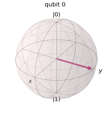
(here and in the sequel, we assume that errors are actually corrected and not just detected to simplify our calculations) on which all stabilizers act trivially, and starting with the next round of measurements, we exclude a Zf operator from the measurements.
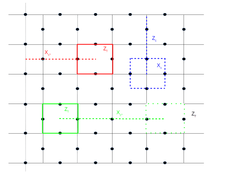
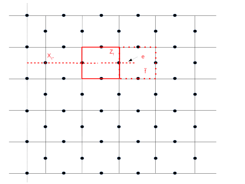
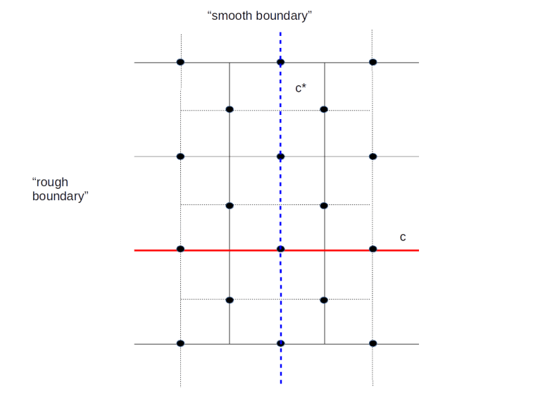
Holes

Of course, this will enlarge the code space. Specifically, let us take a look at the upper left corner of the figure above. Here we have marked a face f and an operator Xc* coming from a string connecting this face with the rough boundary. Then the boundary of c* consists of one point in the dual lattice (the center of f), and hence every face operator commutes with Xc*, except Zf which anti-commutes. If we now define our code space to be the space fixed by all the vertex operators Xv and all face operators except Zf, then Xc* and Zf map that code space to itself. As c* intersects the boundary of f in one point, Zf and Xc* anti-commute and therefore define a set of logical Pauli operators, acting on the code space. Thus we have constructed a logical qubit!

Intuitively, removing the face operator Zf from the set of stabilizers corresponds to poking a “hole” into the surface, i.e. removing the face f and the data qubit in it. But of course we do not change the physical layout of our device at all – all we do is changing the code space and the set of logical Pauli operators. Our original code space, by the way, still exists, but we will tacitly ignore it and work with our new logical qubit.

This construction has a nice physical interpretation in terms of the particle picture that we have introduced in the post on the toric code. Suppose we create a pair of quasi-particles, supported on f and a second face close to the rough boundary. We have seen that we can move these particles by acting with edge operators Xe on them. Thus, we can move the second face on which the particle lives across the rough boundary and now obtain a particle supported on one face only. This is exactly the configuration which is obtained by acting with the logical Pauli X operator of our newly created logical qubit on the ground state, i.e. these logical qubits correspond to pairs of particles where one particle has been “pushed off” the surface!

As usual, this construction has a counterpart in the dual lattice, as shown on the right of of our diagram. The configuration marked in blue consists of a vertex operator Xv and a string c connecting that vertex to the smooth boundary. We can now remove Xv from the stabilizer, and obtain a pair of logical operators Xv and Zc. This type of logical qubit is called a single X-cut in [2], whereas the first type of qubit considered is a single Z-cut – other authors use the term defects for these logical qubits.

This technique allows us in theory to encode a large number of logical qubits in one surface. However, in practice, the restriction that we need to reach the boundary from each of the faces and vertices that we switch off is restricting our layout options a bit. Fortunately, it turns out that this is not even necessary.

In fact, coming back to the analogy of the quasi-particles, nobody forces us to move the second particle off the surface. To see this, consider the configuration marked in green in the lower part of the diagram above. Here we have removed two stabilizers from the code, the face operator Zf corresponding to the face on the left hand side, and the face operator Zf’ corresponding to the face on the right hand side. This will enlarge our code space by a space of dimension four. However, we now gracefully ignore half of that space and instead work with the space spanned by the Pauli operators Zf and Xc*.

A logical qubit obtained by this construction is called a double Z-cut. Of course, we can again repeat this construction in the dual lattice and obtain a double X-cut (these cuts are also for vegetarians…).

Let’s do the twist – moving and braiding qubits

Again, it is time to recap what we have done so far. We have seen that we can create logical qubits by removing face and vertex operators from the set of stabilizers. We have also seen that we can identify logical Pauli X and Z operators acting on these qubits. We can than, of course, also realize a logical Y as the product ZX. What about other gates? And specifically, what about multi-qubit gates?

It turns out that multi-qubit gates can be realized by moving logical qubits around the surface. To make this term a bit more precise, take a look at the following diagram.

ElementaryMove

Here we consider a logical qubit described by the Pauli operators Xc* and Zf, i.e the face operator Zf has been removed from the set of stabilizers. Adjacent to the face f, there is a face that we denote by \bar{f}. By removing Z_{\bar{f}} (and adding Zf again to the set of stabilizers), we would obtain a different code space – we can think of this different code space as a deformation of the code space given by removing Zf.

We want to describe a process that starts with a state in the code space given by Zf and ends with a state in the code space given by Z_{\bar{f}}. To do this, we manipulate the original state in several steps. First, we measure the Pauli X operator Xe for the physical qubit sitting on the edge e of the dual lattice that connects the centre of f with that of \bar{f} – this is the qubit on which both Z_{\bar{f}} and Zf act. Let us assume for a moment that the outcome of this measurement is one. Next, we do another measurement – this time we measure Zf. This will force the system into an eigenstate of Zf. Let us assume again that the outcome of this measurement is plus one, so that the system is now in the new code space obtained by removing Z_{\bar{f}} instead of Zf from the stabilizer.

This procedure gives us a mechanism to transform a state in the original code space into a state in the new code space. It is not difficult to see (again I refer to my notes for all the details) that this leaves the logical meaning of the state untouched, i.e. this transformation maps a logical one in the old codespace to a logical one in the new code space and the same for a logical zero (in fact, it turns out that we need to modify the Pauli operators a bit for this to work).

Of course we cannot directly compare the states before and after the transformation as they live in different code spaces. That, however, changes if we move a logical state around like this along a closed loop. Then we will obtain a new state which is living in the original code space and can compare it directly to the original state, as in the diagram below.

BraidingZXCut

This diagram shows an example where we move a logical qubit generated by a Z-cut once around a logical qubit generated by an X-cut. If we hit upon the intersection between the loop and the X-cut, we pick up an additional transformation. This is a bit like a coordinate transformation – while we move along the loop, we constantly have to adjust our coordinate system, i.e. the logical Pauli operators, to preserve the logical meaning of the qubit. When we reach the initial position, we now have two coordinate system that we can compare, and we find that we have picked up a non-trivial transformation related to the fact that we cannot contract the loop without passing the hole in the surface creating our logical qubit. If you go through all the transformations carefully (or read my notes where I have tried to work out all the details – it is easy to get confused at this point), you will find that the transformation we pick up constitutes a CNOT gate between the two involved qubits! Thus a CNOT can be realized by moving one logical qubit around the second logical qubit once. This is often visualized by a two-strand braid, as illustrated below.

Braids

We have also seen that the transformation given by such a braiding operation is governed by terms like intersection numbers and contracting loop, i.e. the transformation is topological in nature – a slightly deformed braid or path gives the same result. Therefore this operation has a certain natural protection against faults, it is topologically protected. Unfortunately, the surface code does not allow a representation of a universal set of quantum gates by braids – doing this requires the use of a more sophisticated physical equivalent called non-abelian anyons. For the surface code, for instance, the T gate cannot be represented by topological operations and needs to be implemented using a technique called gate teleportation.

We will not go into details on this, but try to quickly describe the basic idea which is based on the observation that the circuit

gateteleportation1.png

can be used to realize the T gate.

How does this circuit work? The upper qubit is an ancilla qubit that is initialized with the specific state

|0\rangle + e^{i \frac{pi}{4}} |1\rangle

by a process called magic state distillation (see [2] for details). Now a short calculation shows that after applying the CNOT gate, the combined system of both qubits will be in the state

T|\psi \rangle \otimes |0 \rangle + (TX |\psi \rangle) \otimes |1 \rangle

Thus we have successfully transferred the state |\psi \rangle into the first qubit (this is why this and similar circuits are called gate teleportation circuits), but still have a superposition. To remove this superposition, we nown perform a measurement MZ on the second qubit. If the outcome of this measurement is one, the first qubit will be in the state T|\psi \rangle 
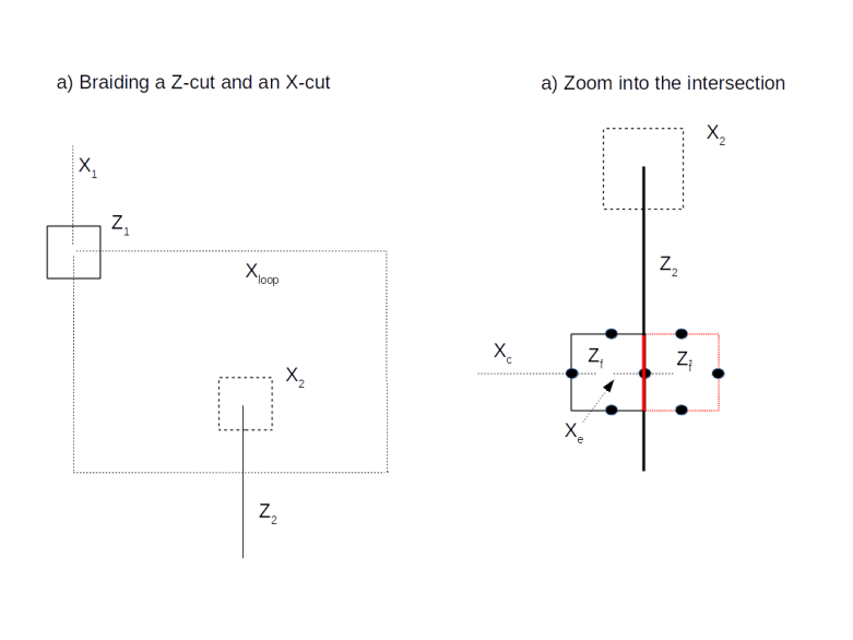
and we are done. If not, i.e. if the measurement results in minus one, then the above formula shows that the resulting state in the first qubit will be TX |\psi \rangle. Now one can easily verify that

TX = X T^*

and

T = S T^*

so that if we apply the sequence SX to the first qubit conditioned on the outcome of the measurement, as indicated in our circuit diagram, the result will in both cases be T|\psi \rangle.

By now, our discussion should have made it clear that the surface codes create a significant overhead. To illustrate this, the appendix of [2] contains an estimation of the number of physical qubits needed to implement Shor’s factoring algorithm for a 2048 bit RSA key. Still, most operations on a surface code are topologically protected, which makes surface codes rather robust. Therefore surface codes remain a promising technology to implement universal fault-tolerant quantum computation, and are one of the most active areas of current research in applied quantum computing.

References

1. S. Bravyi, A. Kitaev, Quantum codes on a lattice with boundary, arXiv:quant-ph/9811052
2. A.G. Fowler, M. Mariantoni, J.M. Martinis, A.N. Cleland, Surface codes: Towards practical large-scale quantum computation, arXiv:1208.0928v2
3. A.G. Fowler, A.M. Stephens, P. Groszkowski, High threshold universal quantum computation on the surface code, arXiv:0803.0272
4. E. Dennis, A. Kitaev, A. Landahl, J. Preskill, Topological quantum memory, arXiv:quant-ph/0110143
5. T.J. Yoder, I.H. Kim, The surface code with a twist, Quantum Vol. 1, 2017 (available online)
6. A. Javadi-Abhari et. al., Optimized Surface Code Communication in Superconducting Quantum Computers, arXiv:1708.09283


Python up an EKS cluster – part I

When you want to try out Kubernetes, you have several choices. You can install Kubernetes in a cluster,  install it locally using Minikube, or use one of the Kubernets offerings of the major cloud providers like AWS, GCP or Azure. In this post, we set up a Kubernetes cluster on Amazons EKS platform. As I love Python, we will do this in two steps. First, we will go through the steps manually, as described in the AWS documentation, using the AWS console. Then, we will learn how to use the AWS Python SDK to automate the recurring steps using Python.

A word of caution before we continue: when you follow these instructions, Amazon will charge you for the cluster as well as for the nodes that the cluster uses! So make sure that you stop all nodes and delete the cluster if you are done to avoid high charges! At the time of writing, Amazon charges 20 cents per hour per cluster plus the EC2 instances underlying the cluster, so if you play with this for one our two hours it will not cost you a fortune, but if you forget to shut everything down and let it run, it can easily add up!

What is EKS?

Before we get our hands dirty, let us quickly discuss what EKS actually is. Essentially, EKS offers you the option to set up a Kubernetes cluster in the Amazon cloud. You can connect to this cluster using the standard Kubernetes API and the standard Kubernetes tools. The cluster will manage worker nodes that are running on Amazons EC2 platform, using your EC2 account. The management nodes on which Kubernetes itself is running are not running on your EC2 instances, but are provided by Amazon.

When you set up an EKS cluster, the cluster and your worker nodes will be running in a virtual private network (VPC). You can add load balancers to make your services reachable from the internet. In addition, EKS is integrated with Amazons IAM.

This tutorial assumes that you own an AWS account and that you have followed the instructions in the IAM getting started guide to set up an IAM user with administrator privileges. Please make sure that you are logged into the AWS console with this IAM user, not your root account.

To set up an EKS cluster, several preparational steps are required. First, you will need to set up an IAM role that EKS will use to control EC2 nodes on your behalf. Next, you will need a VPC in which your cluster will run. After these one time preparation steps have been completed, you can create a Kubernetes cluster, add worker nodes and start deployments. In the following, we will go through most of these steps one by one.

One time preparational steps

Before you can use EKS, you will need to add an IAM role. To do this, navigate to the EKS console (note that this link will automatically take you to your home region). As described on the Getting started with EKS page, open the IAM management console. In the menu on the left, chose “Roles” and then hit the button “Create role”. Choose “EKS” from the list of services and hit “Next: permissions” and then immediately “Next: tags” and “Next: Review”. As the role name, enter “EKSEC2UserRole” (you could of course choose any name you want, but to make the scripts that we will establish further below work, choose this name for this tutorial). At this point, your screen should look as follows.

Screenshot from 2019-03-04 20-49-29

Now confirm the setup of the new role with “Create role” and observe how the new role appears in the list in your IAM console.

The next ingredient that we need is the VPC in which the cluster will be running. To set this up, navigate to the CloudFormation page. Hit the button “Create new stack”. Select “Specify an Amazon S3 template URL” and enter https://amazon-eks.s3-us-west-2.amazonaws.com/cloudformation/2019-02-11/amazon-eks-vpc-sample.yaml
. Then hit “Next”.

On the next page, you will have to choose a stack name. Again, this can be any name, but let us follow the standard suggestion and call it “eks-vpc”. Then hit “Next” twice and then “Create”. AWS will now create the VPC for you, which might take a few minutes, you should see a screen as below while this is in progress.

Screenshot from 2019-03-04 20-57-24

Once the stack has been created, open the “Outputs” tab and record the value of SecurityGroups, VpcID and SubnetIds. . In my case, the values are

Key Value
SecurityGroups sg-005cf103994878f27
VpcId vpc-060469b2a294de8bd
SubnetIds subnet-06088e09ce07546b9,
subnet-0e4a8fd662faadab6,
subnet-0d88f92baecced563

Next, there is some software that you need on your PC. Please follows the instructions on the Getting started with EKS page to download and install kubectl, the aws-iam-authenticator and the aws CLI your your platform. On my Ubuntu Linux PC, this was done using the steps below.

$ sudo snap install kubectl --classic
$ curl -o aws-iam-authenticator https://amazon-eks.s3-us-west-2.amazonaws.com/1.11.5/2018-12-06/bin/linux/amd64/aws-iam-authenticator
$ curl -o aws-iam-authenticator.sha256 https://amazon-eks.s3-us-west-2.amazonaws.com/1.11.5/2018-12-06/bin/linux/amd64/aws-iam-authenticator.sha256
$ openssl sha1 -sha256 aws-iam-authenticator
$ cat aws-iam-authenticator.sha256 # compare checksums!
$ chmod +x ./aws-iam-authenticator
$ mv aws-iam-authenticator $HOME/Local/bin # replace by your local bin directory
$ pip3 install awscli --upgrade --user

Note that pip will install the AWS CLI in $HOME/.local/bin, so make sure to add this directory to your path. We can now test that all tools have been installed by entering

$ kubectl help
$ aws --version

At this point, the aws tool is not yet hooked up with your credentials. To do this, make sure that you have access to the IAM access key ID and access secret key (that you can generate at the IAM console) for your IAM admin user. Then run

$ aws configure

Enter the keys and the required configuration information. When done, enter

$ aws sts get-caller-identity

to confirm that you now access the AWS API with the admin user.

Creating a cluster and adding worker nodes using the AWS console

After all these preparations – which we of course have to go through only once – we are now in a position to create our first EKS cluster. For that purpose, go to the EKS console and look for the box called “Create EKS cluster”. Enter a cluster name – I have chosen “myCluster” (yes, I am very creative) – and hit the button “Next step”.

This will take you to a configuration page. On this page, you will have to select an IAM role that the cluster will use to operate EC2, a VPC and a security group. Make sure to select those entities that we have set up above! Then hit “Create”.

Your cluster will now be created, and you should be taken to the EKS cluster overview page that lists all your clusters along with their status.

EKS_Cluster_Overview

Creation of a cluster can take a few minutes, be patient. At some point, the status of your cluster should switch to active. Congratulations, you are now proud owner of a running Kubernetes cluster!

However, this Kubernetes cluster is pretty useless – there are no worker nodes yet, and you are not yet able to communicate with your cluster using kubectl. We will create worker nodes and run services in the next post. To fix the second problem, we will have to hook up the IAM credential chain used by the AWS CLI tool with kubectl. To do this, enter

$ aws eks --region eu-central-1 update-kubeconfig --name myCluster

Once this has completed, you should now be able to user kubectl to connect to your cluster. As an example, run

$ kubectl get svc
NAME         TYPE        CLUSTER-IP   EXTERNAL-IP   PORT(S)   AGE
kubernetes   ClusterIP   10.100.0.1           443/TCP   6m

Creating a cluster automatically using the Python SDK

Creating a cluster using the EKS console is a bit time consuming, and given the fact that Amazon will charge you for a running cluster, you will want to delete your cluster when you are done and recreate it easily when you need it again. For that purpose, it is very useful to be able to create a cluster using Python.

To do this, let us first delete the cluster again (on the cluster overview page in the EKS console) that we have just created, and compose a Python script that recreates the cluster for us.

First, of course, we need to install the Python SDK Boto3. This is as easy as

$ pip3 install boto3

Note that the SDK uses the same credentials as the AWS CLI, so you still need to go through the steps above to install and configure the AWS CLI.

Our script will accept the name of a cluster (which was myCluster in the example above). It will then need to determine the IAM role, the VPC and subnets and the security group as we did it for the manual setup.

To determine the IAM role, we need an IAM client and use its method get_role to get role details and obtain the role ARN.

iam = boto3.client('iam')
r = iam.get_role(RoleName=eksRoleName)
roleArn = r['Role']['Arn']

Here we assume that the Python variable eksRoleName contains the name of the role that we have created as part of our one time setup.

Getting the VPC ID, the subnet IDs and the security group is a bit more tricky. For that purpose, we will refer back to the CloudFormation stack that we have created as part of our one-time setup. To get the VPC ID and the security group, we can use the following code snippet.

cloudFormation = boto3.client('cloudformation')
r = cloudFormation.describe_stack_resources(
       StackName = "eks-vpc",
       LogicalResourceId="VPC")
vpcId = r['StackResources'][0]['PhysicalResourceId']
r = cloudFormation.describe_stack_resources(
       StackName = "eks-vpc",
       LogicalResourceId="ControlPlaneSecurityGroup")
secGroupId = r['StackResources'][0]['PhysicalResourceId']

Once we have this, we can easily obtain the subnet IDs using the EC2 interface.

ec2 = boto3.resource('ec2')
vpc = ec2.Vpc(vpcId)
subnets = [subnet.id for subnet in vpc.subnets.all()]

We now have all the configuration data that we need to trigger the actual cluster setup. For that purpose, we will create an EKS client and call its method create_cluster, passing the information that we have collected so far as arguments. We then create a waiter object that is polling until the cluster status changes to “Active”.

eks = boto3.client("eks")
response = eks.create_cluster(
               name="myCluster",
               version="1.13",
               roleArn = roleArn,
               resourcesVpcConfig = {
                 'subnetIds' : subnets,
                 'securityGroupIds' : [secGroupId]})
waiter = eks.get_waiter("cluster_active")
waiter.wait(name="myCluster")

When this call completes, our cluster is created. However, we still have to update our Kubernetes configuration file. Of course, we could simply call the AWS CLI, but doing this in Python is more fun. The configuration file that the AWS CLI creates is stored in your home directory, in a subdirectory called kube, and formatted in the simplified markup language known as YAML. Inspecting this file, it is not difficult to translate this into a structure of Python dictionaries and lists, which contains four cluster-specific pieces of data.

  • The cluster endpoint – this is the URL used by kubectl to submit an API call
  • The Amazon resource name of your cluster (ARN)
  • the cluster name
  • a certificate used by kubectl to authorize requests

This information can be retrieved using the method describe_cluster of the EKS client and assembled into a Python data structure. We can then use the Python module yaml to turn this into a string in YAML format, which we can then write to disk. I will not go into detail, but you might want to take a look at the complete script to create a cluster on my GitHub page.

We are now able to automatically create a Kubernetes cluster and connect to it using kubectl. In the next post, we will add the meat – we will learn how to spin up worker nodes and deploy our first pods.


Quantum error correction: an introduction to toric codes

While playing with the IBM Q experience in some of my recent posts, we have seen that real qubits are subject to geometric restrictions – two-qubit gates cannot involve arbitrary qubits, but only qubits that are in some sense neighbors. This suggests that efficient error correction codes need to tie to the geometry of the quantum device. Toric codes are an example of these codes that create interesting connections between topology and quantum computing.

The stabilizer group of a toric code

In their original form introduced by A. Kitaev in 1997 (see e.g. [1]), toric codes are designed to operate on quantum circuits arranged on a torus. Specifically, we consider a 2-dimensional discrete lattice L with periodic boundary conditions. On each edge of this lattice, we place exactly one qubit.

In algebraic topology, one can associate with such a lattice an abelian group called the group of one-chains of the lattice and denoted by C_1(L)
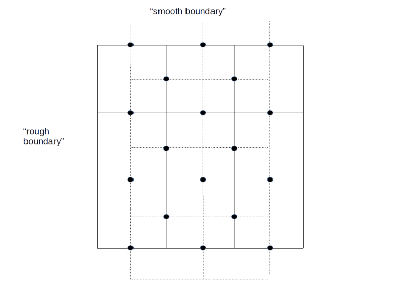
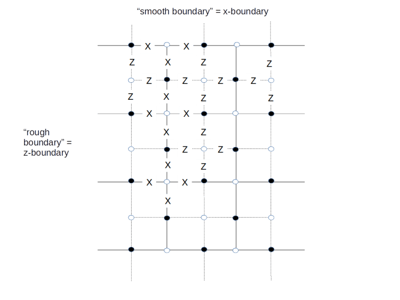
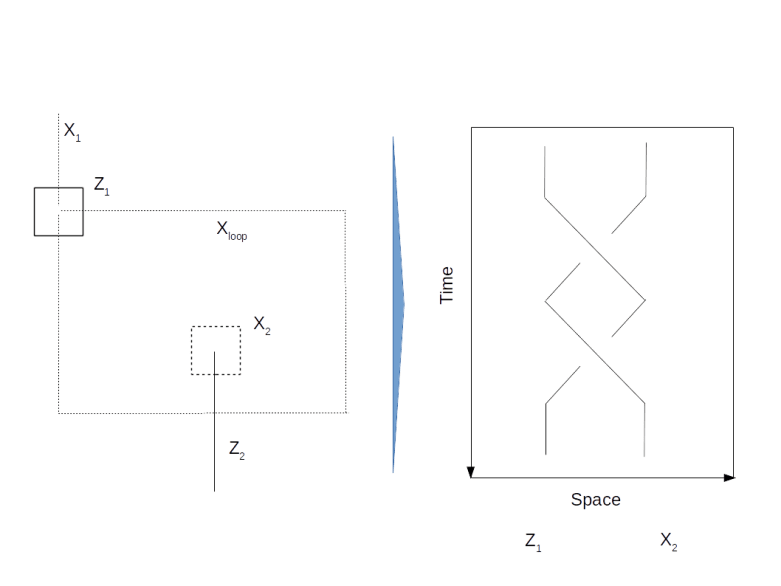
. The elements of this group are simply binary linear combinations of edges, i.e. subsets of all edges. Addition in this group is given by joining the subsets, while dropping elements that appear twice. As there is one qubit sitting on every edge, every chain c, i.e. every subset of edges, will yield an operator that we call Xc and which is simply given by applying the Pauli X operator to each of the qubits sitting on an edge appearing in c. Similarly, one can define an operator Zc for evey chain c by combining the Pauli Z operators for the qubits touched by c.

This sounds a bit daunting and formal, so time to look at a picture and a few examples.

ToricCode

This diagram shows a graphical representation of our lattice L. The solid lines represent the edges of the lattice, their intersections are the vertices, see the labels at the lower right corner of the image. Cornered by four vertices and surrounded by four edges, there are the faces of the lattice. The black dots in the diagram indicate the qubits on the lattice.

Now let us look at the face marked in red and labeled by f at the top of the diagram. This face is surrounded by four edges colored red as well whose union is called the boundary of the face. This boundary is formalized as a one-chain denoted by \partial f \in C_1(L)
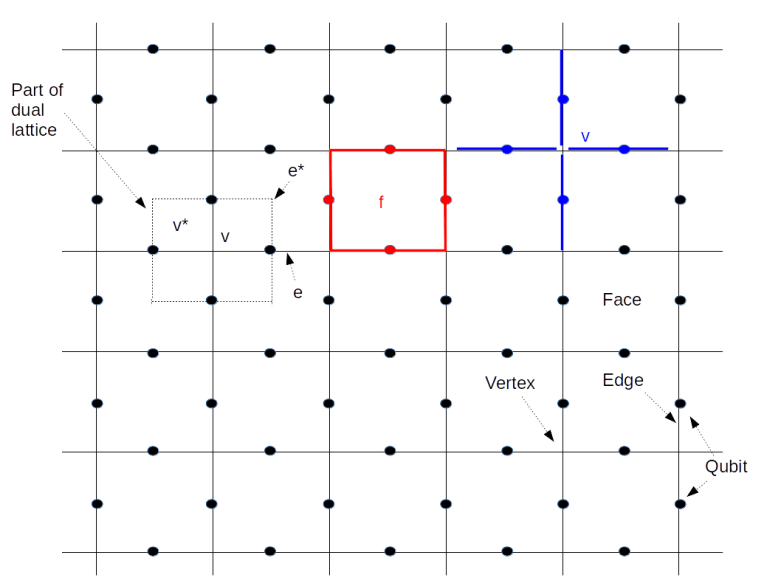
. As described above, we can associate an operator Z_{\partial f} to this one chain, which is simply given by letting a Pauli Z operator act on each of the qubits sitting on the red edges. This operator is called the face operator associated with the face f and denoted by Zf

On the right of the face, we have – in blue – marked a single vertex v. This vertex again defines a chain, namely the subset of all edges – marked in blue – that touch the vertex. Again, we can associate an operator to this chain, this time we choose the product of the Pauli X operators acting on the qubits on the blue edges. This operator is called the vertex operator for the vertex v and denoted by Xv.

Our lattice has many faces and many vertices. For each face, we have a face operator and for each vertex, we have a vertex operator. It is not difficult to check that all these operators do in fact commute (note that a vertex touches every boundary twice). Therefore the group S generated by all these operators is an abelian group.

Now recall from one of my previous posts that the stabilizer formalism can be used to associate to every abelian subgroup of the Pauli group a code. The code obtained from the group S generated by all face and vertex operators is called the toric code.

Let us try to better understand the code space TS. Suppose that our lattice has E edges, V vertices and F faces. Then there are E qubits, i.e. the Hilbert space of physical qubits has dimension 2E. The stabilizer group is generated by the V vertex operators and the F face operators, i.e. by V + F elements. However, these elements are not independent – there are relations imposed by the toric geometry. In fact, the product of all vertex operators is one and the product of all face operators is one (this is easiest seen with a bit of background in algebraic topology – for those readers who have that background, I refer to my notes on quantum error correction for the mathematical details behind this and some other statements in this post). Thus there are in fact V + F – 2 generators. As each generator introduces a constraint on the code space that cuts the Hilbert space dimension down by a factor two, the dimension of the code space is

2E – (V+F – 2) = 22 – (V + F – E)

Now the number V + F – E is known as the Euler number of the torus in algebraic topology, and it also known that the Euler number of the torus is zero. Therefore the dimension of the code space is 22 = 4, i.e. the code space encodes two logical qubits (this will change if we later move on to a planar geometry).

Let us now try to understand the logical gates acting on these two logical qubits. By the general theory of stabilizer codes, we know that the logical operators are those operators that commute will all elements in the stabilizer. What does this mean geometrically? To see this, consider the following diagram.

ToricCodeLogicalPauliMatrices

Consider the vertical red line in the diagram, labeled by c1. This line is a subset of edges, i.e. a one chain. To this chain, we can associate a Z operator Zc1, which is the product of all Pauli Z operators acting on the qubits touched by the red line. Being a Z operator, this operator commutes with all face operators. What about the vertex operators?

Close to the right border of the lattice, we have indicated the vertex operator Xv associated with the vertex v. This vertex operator acts on four qubits, indicated by the edges marked with the blue dashed line. Two of these edges also appear in the chain c1. Therefore, when we commute Xv and Zc1, we pick up two signs that cancel and the operators commute. Thus Zc1 commutes with all vertex and face operators and is in the normalizer. The same is true for the operator associated with the second red line. These two Z operators therefore act on the logical qubit. By convention, we can define the logical state |0 \rangle_L 
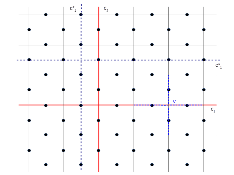
to be the state which is left invariant by these two operators.

It is interesting to note that the vertex operator Xv commutes with Zc1 because the chain c1 crosses the vertex v and therefore contains both edges touching v. If however, a chain c ends at v, then we will only pick up one sign when commuting the X past the Z operators. Geometrically, a vertex operator Xv anti-commutes with a Z-operator Zc associated with a chain c if and only if the vertex v is in the boundary of c, otherwise it commutes. The red line in our diagram is distinguished by the fact that its boundary is empty – it is a closed circle or a cycle in the language of algebraic topology that goes around the torus once. It therefore commutes with all vertex operators and thus is an element of the stabilizer.

Similarly, the dotted blue lines represent X operators, given by the product of the Pauli X operators acting on those qubits intersected by the blue line. A similar argument shows that, as these lines also go once around the torus, the X operators associated with them are in the normalizer of S as well. Thus we obtain two X operators that act as logical Pauli X operators on our code space. Given the logical X and Z operators, we can therefore implement all single qubit gates on our code space. It turns out that multi-qubit gates can be implemented by braid operations, but we will leave this to a later post when we study planar codes.

The particle interpretation of the toric code and anyons

Let us now turn to the particle interpretation of error correction in these codes, that will bring the famous anyons and ideas from topological quantum computing into play. For that purpose, consider the operator

H = - \sum_v X_v - \sum_f Z_f

which is the sum of all face and vertex operators. Clearly, this operator is hermitian, and can therefore be thought of as the operator of a physical system. Does this system have a particle interpretation?

To see this, let us try to determine the eigenstates of the Hamiltonian, i.e. the energy levels of our system. As the Xv and the Zf all commute, we can find a simultaneous basis of eigenstates that will diagonalize the Hamiltonian. Let us call this basis \{ |\psi_i \rangle \}. Each of these vectors is an eigenstate of all face and vertex operators, and we denote the corresponding eigenvalues by xvi and zfi. Clearly, |\psi_i \rangle is then an eigenvector of H with eigenvalue

- \sum_f z_{fi} - \sum_v x_{vi}

This is minimal if and only if all the xvi and zfi are equal to one, which is the case if |\psi_i \rangle is an element of the code space. Thus we have identified the elements of the code space as the ground states of our system!

Now let us introduce an error into our system. One way to do this is to pick a chain c, i.e. a path on the lattice, and apply the Zc operator to one of the ground states |g \rangle. Let us try to determine the error syndrome of this state, i.e. let us try to figure out for which elements of the stabilizer, this state is no longer in the +1 eigenspace.

As all Z operators commute, the state is clearly still in the +1 eigenspace of all the face operators Zf. If Xv is a vertex operator, the state will be in the -1 eigenspace if and only if Zc anti-commutes with Xv. But we have already seen that this happens if and only if v is in the boundary of c, i.e. v is one of the two vertices where the path c starts and ends! Thus the error syndrome is localized at those two vertices – if we imagine the vertex operator measurements as being signaled by green (outcome plus one) and red (outcome minus one) lights attached to the respective vertex, the error would be represented two red lights sitting at these vertices.

If we now expand the state Z|g \rangle into eigenstates of the Hamiltonian, the above discussion shows that the eigenvalue has increased by four. Thus errors correspond to excited states, and the operators Zc are creation operators that create excited states that are in a certain sense localized at the vertices of the lattice. It is tempting and common to therefore call these excitations quasi-particles, similar to the phonons in a crystal lattice.
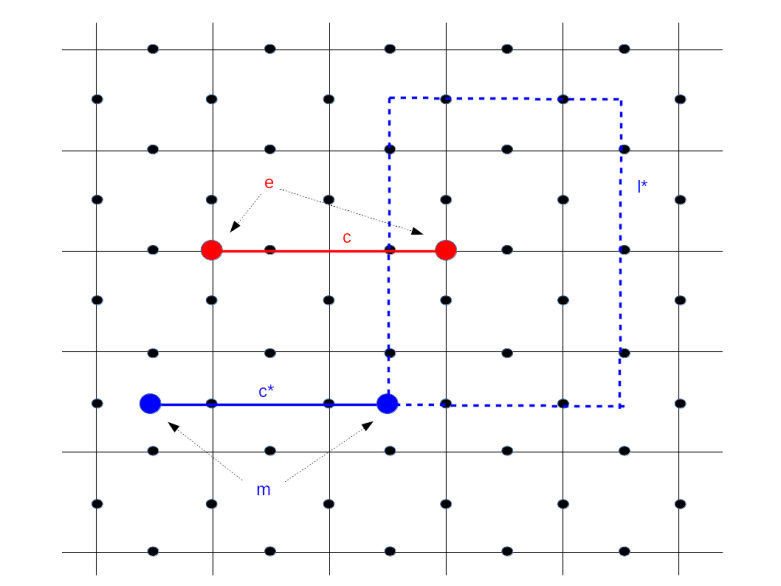
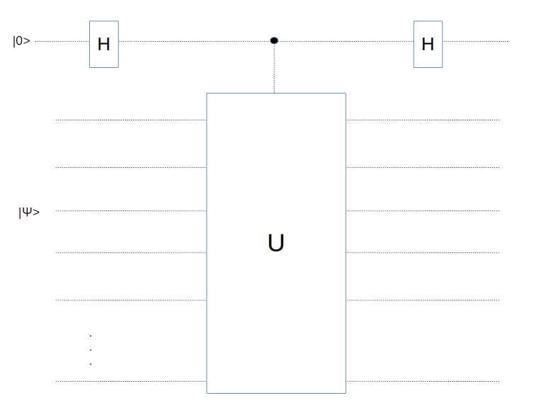
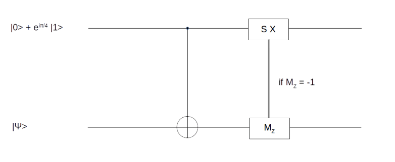
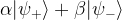
So far we have associated an error operator Zc and therefore a particle with every chain, i.e. a path that runs along the edges. We can also consider a path that runs perpendicular to all the edges – in algebraic topology, this would be called a chain in the dual lattice or a co-chain. To every such path, we can associate an X operator, and this X operator acting on a ground state will create another excitation. The particles associated with a chain is called an electric charge e by Kitaev, and the particle created by a co-chain is called an magnetic vortex m.

Anyons

As indicated in the diagram above, electric charges come in pairs, are located on vertices of the lattice and manifest themselves as -1 eigenvalues of the corresponding vertex operators, whereas magnetic particles live on pairs of faces of the vertex and appear as -1 eigenvalues of face operators. In this diagram, the solid red line creates a pair of electric particles, and the solid blue line creates a pair of magnetic particles.

How do these particles relate to the composition of chains? Suppose that we are given a chain c12 running from vertex 1 to vertex 2 and a second chain c23 running from vertex 2 to vertex 3. Then there are two ways to create the particle sitting at the vertices 1 and 3 – we can either first act with the Z operator associated with the chain c12 and then let the operator associated with the chain c23 act, or we can form the sum c13 of the chains which now runs from 1 to 3 and let the operator associated with this chain act. Of course, the result will be the same. Thus we can interpret the act of applying the operator given by the chain c23 to an excited state as moving one of the particles from vertex 2 to vertex 3. The same applies to magnetic particles.

Now let us again consider the image above. Look at the blue dashed loop. According to what we have just said, we can start with the particle pair created by the solid blue line and then move one of the particles around that closed loop. The result will be a particle pair living at the same location as the original pair. You might think that the new state is in fact identical to the old state, but this is not true – the state picks up a phase factor minus one. This is the reason why Kitaev calls our quasi-particles anyons, a term generally used in particle physics to characterize particles with non-trivial statistics (in our case, mutual statistics)

Exchanging particles by moving them around each other can be described as an action of the pure braid group, i.e. as an action of the group of braids that return each particle to its original position (this subgroup, the kernel of the natural homomorphism from the braid group to the permutation group, is sometimes called the group of colored braids). If we perturb a braid slightly, the action will remain unchanged, so the unitary operators which are given by that action are by construction rather stable in the presence of noise. In [1], Kitaev developed the idea to use braid group representations to implement quantum gates. Unfortunately, the set of operators that we can obtain in this way using the toric code is not sufficient to implement a universal quantum computer – we will get back to this point in a later post when we look at the actual procedures used to perform computations in a toric or surface code. Therefore Kitaev goes on to describe certain hypothetical particles called non-abelian anyons which, if they can be physically realized, provide sufficiently rich unitary operations. This approach is called topological quantum computation. We will not go into further details but refer to the original work [1].

Measurement and error correction for toric codes

Let us quickly summarize what we have found so far. The code space of a toric code can be thought of as the ground state of a physical system, describing a collection of two-state systems located on the edges of a lattice. Errors correspond to fundamental excitations, i.e. quasi-particles, that come in pairs and sit on vertices and faces of the lattice. These errors can be detected by measuring face and vertex operators.

How can we perform these measurements in practice? To understand this, let us first recall a general approach for measuring eigenvalues. Suppose that U is an operator that is hermitian and at the same time unitary. Consider the following circuit which is a combination of two Hadamard gates with a controlled-U operation.

ControlledUMeasurement

Let us calculate the state after applying this circuit. The initial state is

|0 \rangle |\psi \rangle

After applying the Hadamard gate to the first qubit, we obtain

\frac{1}{\sqrt{2}} \big[ |0 \rangle |\psi \rangle  + |1 \rangle |\psi \rangle   \big]

which the controlled U operation turns into

\frac{1}{\sqrt{2}} \big[ |0 \rangle \otimes |\psi \rangle  +  |1 \rangle \otimes U |\psi \rangle  \big]

Now U is unitary, and therefore its eigenvalues are plus and minus one. So we can decompose our state |\psi \rangle as

\alpha |\psi_+ \rangle + \beta |\psi_- \rangle

where |\psi_+\rangle is an eigenstate with eigenvalue plus one and |\psi_-\rangle an eigenstate with eigenvalue minus one. Plugging this into the above equation and applying the final Hadamard operator shows that the final outcome of the circuit will be

\alpha |0 \rangle \otimes |\psi_+\rangle + \beta |1 \rangle \otimes |\psi_- \rangle

If we now apply a measurement to the control qubit, which serves as an ancilla here, the state is projected onto either |1 \rangle \otimes |\psi_- \rangle or |0 \rangle \otimes |\psi_+ \rangle, with probabilities |\beta|^2 and |\alpha|^2. The remaining qubits end up in the state |\psi_-\rangle or |\psi_+ \rangle, i.e. in an eigenstate. Thus applying this circuitry and measuring the ancilla has the same implications as measuring the operator U and yields the same information.

Let us now apply this idea to the problem of measuring one of the operators Xv. This operator is a tensor product of four \sigma_x operators, i.e. inversion operators. Therefore a controlled-Xv circuit is nothing but a sequence of controlled inversions, i.e. CNOT gates. Thus we can measure a vertex operator using the following circuit.

MeasuringXfI

Here the four qubits at the bottom correspond to the four edges meeting the vertex v. So we need one ancilla qubit for doing the measurement, and we need to be able to combine it in gates with all the four qubits sitting on the edges meeting v. For the physical implementation, the easiest approach is to place this additional qubit called measurement qubit in the vertex itself, in contrast to the data qubits that we have already placed on the edges. So we add one data qubit to each vertex.

A circuit along the same lines can be constructed to measure Zf for a face f. Using that H \sigma_x H = \sigma_z
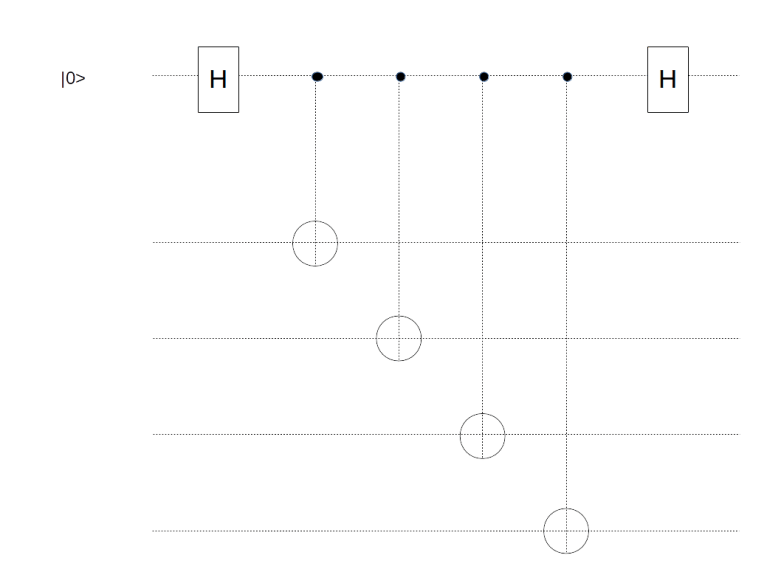
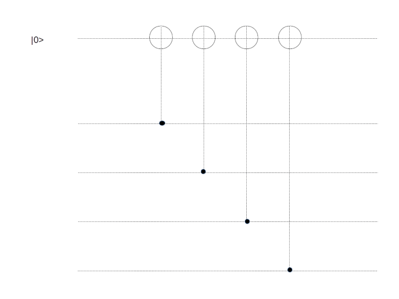
, we can construct such a circuit as follows. In the first time step, apply a Hadamard to both the ancilla and all target qubits. Then apply CNOT operators to all target qubits, controlled by the ancilla, and then apply Hadamard operators again. Now, it is well known that conjugating the CNOT with Hadamard gates switches the roles of target qubits and control qubits. This gives us the circuit displayed below.
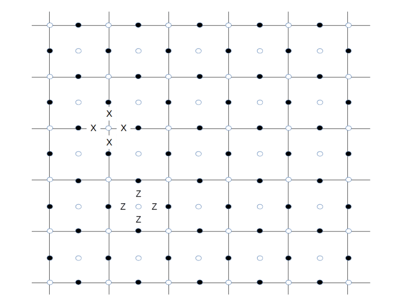
MeasuringZv

Again, for each face f, we need an ancilla qubit to measure Zf. This qubit will have to interact with all data qubits on the edges bounding this face, so it is easiest to position it in the center of that face.

Overall, we have now added F + V measurement qubits to our original E data qubits. Now the Euler characteristic of the torus is zero, and therefore F + V = E, showing that this procedure actually doubles the number of physical qubits.

We have now arrived at a description of the toric code (and its cousin the surface code) that one can often find as a definition in the literature but which somehow obscures the relation to the surface topology a bit.

  • We start with a lattice L with E edges and identify opposite borders
  • On each vertex, we place a data qubit
  • On each face, we place a measurement qubit called a Z-qubit
  • On each vertex, we place a measurement qubit called an X-qubit
  • To each X-qubit, we associate the operator that acts as a bit flip on the four data qubits next to the measurement qubit
  • To each Z-qubit, we associate the operator that acts a a phase flip on the four data qubits next to the measurement qubit

Thus every data qubit is acted on by four operators, the two Z-operators corresponding to the adjacent faces and the two X-operators corresponding to the adjacent vertices. The additional measurement qubits – indicated by white circles in contrast to the dark circles being the data qubits – are shown below.

ToricCodeMeasurementQubits

For one face and one vertex, we have indicated the associated operators Xv and Zf by adding letters X and Z to show how these operators act on the nearby data qubits. This is the graphical representation typically used in the literature (like [3]). Note that some authors use different conventions and associate Z-operators with faces and X-operators with vertices, but this is of course completely equivalent due to the duality relations between a lattice and a dual lattice.

This completes our short introduction to toric codes. In the next post in my series on quantum error correction, we will pass on to a planar geometry which turns the toric code into a surface code.

References

1 A. Kitaev, Fault-tolerant quantum computation by anyons, arXiv:quant-ph/9707021
2. H. Bombin, An introduction to topological quantum codes, in Quantum error correction, edited by D.A. Lidar and T.A. Brun, Cambridge University Press, New York, 2013, available as arXiv:quant-ph/1311.0277
3. A.G. Fowler, M. Mariantoni, J.M. Martinis, A.N. Cleland, Surface codes: Towards practical large-scale quantum computation, arXiv:1208.0928v2

Kubernetes – an overview

Docker containers are nice and offer a very lean and structured way to package and deploy applications. However, if you really want to run large scale containerized applications, you need more – you need to deploy, orchestrate and manager all your containers in a highly customizable and automated way. In other words, you need a container management platform like Kubernetes.

What is a container management platform?

Imagine you have a nice, modern application based on microservices, and you have decided to deploy each microservice into a separate container. Thus your entire application deployment will consist of a relatively large number, maybe more than hundred, individual containers. Each of these containers needs to be deployed, configured and monitored. You need to make sure that if a container goes down, it is restarted and traffic is diverted to a second instance. You need to distribute your load evenly. You need to figure out which container should run on which virtual or physical machine. When you upgrade or deploy, you need to take dependencies into account. If traffic reaches a certain threshold, you would like to scale, either vertically or horizontally. And so forth…

Thus managing a large number of containers in a production-grade environment requires quite some effort. It would be nice to have a platform that is able to

  • Offer loadbalancing, so that incoming traffic is automatically routed to several instances of a service
  • Easily set up container-level networks
  • Scale out automatically if load increases
  • Monitor running services and restart them if needed
  • Distribute containers evenly across all nodes in your network
  • Spin up new nodes or shut down nodes depending on the traffic
  • Manage your volumes and storage
  • Offer mechanisms to upgrade your application and the platform and / or rollback upgrades

In other words, you need a container management platform. In this post – and in a few following posts – I will focus on Kubernetes, which is emerging as a de facto standard for container management platforms. Kubernetes is now the underlying platform for industry grade products like RedHat OpenShift or Rancher, but can of course be used stand-alone as well. In addition, all major cloud providers like Amazon (EKS), Google (GKE), Azure (AKS) and IBM ( IBM Cloud Kubernetes Service) offer Kubernetes as a service on their respective platforms.

Basic Kubernetes concepts

When you first get in touch with the world of Kubernetes, the terminology can be a bit daunting – there are pods, clusters, services, containers, namespaces, deployments, and many other terms that will be thrown at you. Time to explain some of the basic concepts very high level – we will get in closer contact with most of them over the next few posts.

The first object we need to understand is a Kubernetes node. Essentially, a node is a compute ressource, i.e. some sort of physical or virtual host on which Kubernetes can run things. In a Kubernetes cluster, there are two types of nodes. A master node is a node on which the Kubernetes components itself are running. A worker node is a node on which application workloads are running.

On each worker node, Kubernetes will start several agents, for instance the kubelet which is the primary agent responsible for controlling a node. In addition to the agent, there are of course the application workloads. One might suspect that these workloads are managed on a container basis, however, this is not quite the case. Instead, Kubernetes groups containers into objects called pods. A pod is the smallest unit handled by Kubernetes. It encompasses one or more containers that share resources like storage volumes, network namespaces and the same lifecycle. It is quite common to see pods with only one application container, but one might also decide to put, for instance, a microservice and a database into one pod. In this case, when the pod is started, both containers (the container containing the microservice and the container containing the database) are brought up on the same node, can see each other in the network under “localhost” and can access the same volumes. In a certain sense, a pod is therefore a sort of logical host on which our application containers run. Kubernets assigns IP addresses to pods, and applications running in different pods need to use these IP addresses to communicate via the network.

When a user asks Kubernetes to run a pod, a Kubernetes component called the scheduler identifies a node on which the pod is then brought up. If the pod dies and needs to be restarted, it might be that the pod is restarted on a different node. The same applies if the node goes down, in this case Kubernetes will restart pods running on this container on a different node. There are also other situations in which a pod can be migrated from one node to a different node, for instance for the purpose of scaling. Thus, a pod is a volatile entity, and an application needs to be prepared for this.

KubernetesBasics

Pods themselves are relatively dumb objects. A large part of the logic to handle pods is located in componentes called controllers. As the name suggests, these are components that control and manage pods. There are, for instance, special controllers that are able to autoscale the number of pods or to run a certain number of instances of the same pod – called replicas. In general, pods are not started directly by a Kubernetes user, but controllers are defined that manage the pods life cycle.

In Kubernetes, a volume is also defined in the context of a pod. When the pod ceases to exist, so does the volume. However, a volume can of course be backed by persistent storage, in which case the data on the volume will outlive the pod. On AWS, we could for instance mount an EBS volume as a Kubernetes volume, in which case the data will persist even if we delete the pod, or we could use local storage, in which case the data will be lost when either the pod or the host on which the pod is running (an AWS virtual machine) is terminated.

There are many other objects that are important in Kubernetes that we have not yet discussed – networks, services, policies, secrets and so forth. This post is the first in a series which will cover most of these topics in detail. My current plans are to discuss

Thus, in the next post, we will learn how to set up and configure AWS EKS to see some pods in action (I will start with EKS for the time being, but also cover other platforms like DigitalOcean later on).