Python – Page 3 – LeftAsExercise

Automating provisioning with Ansible – variables and facts

In the playbooks that we have considered so far, we have used tasks, links to the inventory and modules. In this post, we will add another important feature of Ansible to our toolbox – variables.

Declaring variables

Using variables in Ansible is slightly more complex than you might expect at the first glance, mainly due to the fact that variables can be defined at many different points, and the precedence rules are a bit complicated, making errors likely. Ignoring some of the details, here are the essential options that you have to define variables and assign values:

You can assign variables in a playbook on the level of a play, which are then valid for all tasks and all hosts within that play
Similarly, variables can be defined on the level of an individual task in a playbook
You can define variables on the level of hosts or groups of hosts in the inventory file
There is a module called set_fact that allows you to define variables and assign values which are then scoped per host and for the remainder of the playbook execution
Variables can be defined on the command line when executing a playbook
Variables can be bound to a module so that the return values of that module are assigned to that variable within the scope of the respective host
Variable definitions can be moved into separate files and be referenced from within the playbook
Finally, Ansible will provide some variables and facts

Let us go through these various options using the following playbook as an example.

---
- hosts: all
  become: yes
  # We can define a variable on the level of a play, it is
  # then valid for all hosts to which the play applies
  vars:
    myVar1: "Hello"
  vars_files:
  - vars.yaml
  tasks:
    # We can also set a variable using the set_fact module
    # This will be valid for the respective host until completion
    # of the playbook
  - name: Set variable
    set_fact:
      myVar2: "World"
      myVar5: "{{ ansible_facts['machine_id'] }}"
    # We can register variables with tasks, so that the output of the
    # task will be captured in the variable
  - name: Register variables
    command: "date"
    register:
      myVar3
  - name: Print variables
    # We can also set variables on the task level
    vars:
      myVar4: 123
    debug:
      var: myVar1, myVar2, myVar3['stdout'], myVar4, myVar5, myVar6, myVar7

At the top of this playbook, we see an additional attribute vars on the level of the play. This attribute itself is a list and contains key-value pairs that define variables which are valid across all tasks in the playbook. In our example, this is the variable myVar1.

The same syntax is used for the variable myVar4 on the task level. This variable is then only valid for that specific task.

Directly below the declaration of myVar1, we instruct Ansible to pick up variable definitions from an external file. This file is again in YAML syntax and can define arbitrary key-value pairs. In our example, this file could be as simple as

---
  myVar7: abcd

Separating variable definitions from the rest of the playbook is very useful if you deal with several environments. You could then move all environment-specific variables into separate files so that you can use the same playbook for all environments. You could even turn the name of the file holding the variables into a variable that is then set using a command line switch (see below), which allows you to use different sets of variables for each execution without having to change the playbook.

The variable myVar3 is registered with the module command, meaning that it will capture the output of this module. Note that this output will usually be a complex data structure, i.e. a dictionary. One of the keys in this dictionary, which depends on the module, is typically stdout and captures the output of the command.

For myVar2, we use the module set_fact to define it and assign a value to it. Note that this value will only be valid per host, as myVar5 demonstrates (here we use a fact and Jinja2 syntax – we will discuss this further below).

In the last task of the playbook, we print out the value of all variables using the debug module. If you look at this statement, you will see that we print out a variable – myVar6 – which is not defined anywhere in the playbook. This variable is in fact defined in the inventory. Recall that the inventory for our test setup with Vagrant introduced in the last post looked as follows.

[servers]
192.168.33.10
192.168.33.11

To define the variable myVar6, change this file as follows.

[servers]
192.168.33.10 myVar6=10
192.168.33.11 myVar6=11

Note that behind each host, we have added the variable name along with its value which is specific per host. If you now run this playbook with a command like

export ANSIBLE_HOST_KEY_CHECKING=False
ansible-playbook  \
        -u vagrant \
        --private-key ~/vagrant/vagrant_key \
        -i ~/vagrant/hosts.ini \
         definingVariables.yaml

then the last task will produce an output that contains a list of all variables along with their values. You will see that myVar6 has the value defined in the inventory, that myVar5 is in fact different for each host and that all other variables have the values defined in the playbook.

As mentioned before, it is also possible to define variables using an argument to the ansible-playbook executable. If, for instance, you use the following command to run the playbook

export ANSIBLE_HOST_KEY_CHECKING=False
ansible-playbook  \
        -u vagrant \
        --private-key ~/vagrant/vagrant_key \
        -i ~/vagrant/hosts.ini \
        -e myVar4=789 \
         definingVariables.yaml

then the output will change and the variable myVar4 has the value 789. This is an example of the precedence rule mentioned above – an assignment specified on the command line overwrites all other definitions.

Using facts and special variables

So far we have been using variables that we instantiate and to which we assign values. In addition to these custom variables, Ansible will create and populate a few variables for us.

First, for every machine in the inventory to which Ansible connects, it will create a complex data structure called ansible_facts which represents data that Ansible collects on the machine. To see an example, run the command (assuming again that you use the setup from my last post)

export ANSIBLE_HOST_KEY_CHECKING=False
ansible \
      -u vagrant \
      -i ~/vagrant/hosts.ini \
      --private-key ~/vagrant/vagrant_key  \
      -m setup all

This will print a JSON representation of the facts that Ansible has gathered. We see that facts include information on the machine like the number of cores and hyperthreads per core, the available memory, the IP addresses, the devices, the machine ID (which we have used in our example above), environment variables and so forth. In addition, we find some information on the user that Ansible is using to connect, the used Python interpreter and the operating system installed.

It is also possible to add custom facts by placing a file with key-value pairs in a special directory on the host. Confusingly, this is called local facts, even though these facts are not defined on the control machine on which Ansible is running but on the host that is provisioned. Specifically, a file in /etc/ansible/facts.d ending with .fact can contain key-value pairs that are interpreted as facts and added to the dictionary ansible_local.

Suppose, for instance, that on one of your hosts, you have created a file called /etc/ansible/facts.d/myfacts.fact with the following content

[test]
testvar=1

If you then run the above command again to gather all facts, then, for that specific host, the output will contain a variable

"ansible_local": {
            "myfacts": {
                "test": {
                    "testvar": "1"
                }
            }

So we see that ansible_local is a dictionary, with the keys being the names of the files in which the facts are stored (without the extension). The value for each of the files is again a dictionary, where the key is the section in the facts file (the one in brackets) and the value is a dictionary with one entry for each of the variables defined in this section (you might want to consult the Wikipedia page on the INI file format).

In addition to facts, Ansible will populate some special variables like the inventory_hostname, or the groups that appear in the inventory file.

Using variables – Jinja2 templates

In the example above, we have used variables in the debug statement to print their value. This, of course, is not a typical usage. In general, you will want to expand a variable to use it at some other point in your playbook. To this end, Ansible uses Jinja2 templates.

Jinja2 is a very powerful templating language and Python library, and we will only be able to touch on some of its features in this post. Essentially, Jinja2 accepts a template and a set of Python variables and then renders the template, substituting special expressions according to the values of the variables. Jinja2 differentiates between expressions which are evaluated and replaced by the values of the variables they refer to, and tags which control the flow of the template processing, so that you can realize things like loops and if-then statements.

Let us start with a very simple and basic example. In the above playbook, we have hard-coded the name of our variable file vars.yaml. As mentioned above, it is sometimes useful to use different variable files, depending on the environment. To see how this can be done, change the start of our playbook as follows.

---
- hosts: all
  become: yes
  # We can define a variable on the level of a play, it is
  # then valid for all hosts to which the play applies
  vars:
    myVar1: "Hello"
  vars_files:
  - "{{ myfile }}"

When you now run the playbook again, the execution will fail and Ansible will complain about an undefined variable. To fix this, we need to define the variable myfile somewhere, say on the command line.

export ANSIBLE_HOST_KEY_CHECKING=False
ansible-playbook  \
        -u vagrant \
        --private-key ~/vagrant/vagrant_key \
        -i ~/vagrant/hosts.ini \
        -e myVar4=789 \
        -e myfile=vars.yaml \
         definingVariables.yaml

What happens is that before executing the playbook, Ansible will run the playbook through the Jinja2 templating engine. The expression {{myfile}} is the most basic example of a Jinja2 expression and evaluates to the value of the variable myfile. So the entire expression gets replaced by vars.yaml and Ansible will read the variables defined there.

Simple variable substitution is probably the most commonly used feature of Jinja2. But Jinja2 can do much more. As an example, let us modify our playbook so that we use a certain value for myVar7 in DEV and a different value in PROD. The beginning of our playbook now looks as follows (everything else is unchanged):

---
- hosts: all
  become: yes
  # We can define a variable on the level of a play, it is
  # then valid for all hosts to which the play applies
  vars:
    myVar1: "Hello"
    myVar7: "{% if myEnv == 'DEV' %} A {% else %} B {% endif %}"

Let us run this again. On the command line, we set the variable myEnv to DEV.

export ANSIBLE_HOST_KEY_CHECKING=False
ansible-playbook  \
        -u vagrant \
        --private-key ~/vagrant/vagrant_key \
        -i ~/vagrant/hosts.ini \
        -e myVar4=789 \
        -e myEnv=DEV \
         definingVariables.yaml

In the output, you will see that the value of the variable is ” A “, as expected. If you use a different value for myEnv, you get ” B “. The characters “{%” instruct Jinja2 to treat everything that follows (until “%}”) as tag. Tags are comparable to statements in a programming language. Here, we use the if-then-else tag which evaluates to a value depending on a condition.

Jinja2 comes with many tags, and I advise you to browse the documentation of all available control structures. In addition to control structures, Jinja2 also uses filters that can be applied to variables and can be chained.

To see this in action, we turn to an example which demonstrates a second common use of Jinja2 templates with Ansible apart from using them in playbooks – the template module. This module is very similar to the copy module, but it takes a Jinja2 template on the control machine and does not only copy it to the remote machine, but also evaluates it.

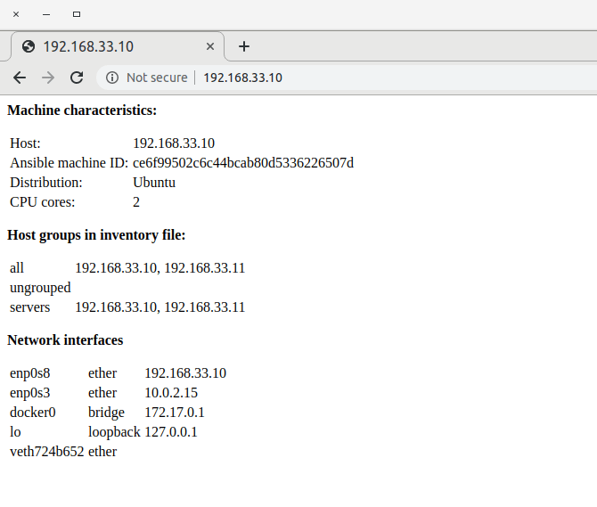
Suppose, for instance, you wanted to dynamically create a web page on the remote machine that reflects some of the machines’s characteristics, as captured by the Ansible facts. Then, you could use a template that refers to facts to produce some HTML output. I have created a playbook that demonstrates how this works – this playbook will install NGINX in a Docker container and dynamically create a webpage containing machine details. If you run this playbook with our Vagrant based setup and point your browser to http://192.168.33.10/, you will see a screen similar to the one below, displaying things like the number of CPU cores in the virtual machine or the network interfaces attached to it.

I will not go through this in detail, but I advise you to try out the playbook and take a look at the Jinja2 template that it uses. I have added a few comments which, along with the Jinja2 documentation, should give you a good idea how the evaluation works.

To close this post, let us see how we can test Jinja2 templates. Of course, you could simply run Ansible, but this is a bit slow and creates an overhead that you might want to avoid. As Jinja2 is a Python library, there is a much easier approach – you can simply create a small Python script that imports your template, runs the Jinja2 engine and prints the result. First, of course, you need to install the Jinja2 Python module.

pip3 install jinja2

Here is an example of how this might work. We import the template index.html.j2 that we also use for our dynamic webpage displayed above, define some test data, run the engine and print the result.

import jinja2
#
# Create a Jinja2 environment, using the file system loader
# to be able to load templates from the local file system
#
env = jinja2.Environment(
    loader=jinja2.FileSystemLoader('.')
)
#
# Load our template
#
template = env.get_template('index.html.j2')
#
# Prepare the input variables, as Ansible would do it (use ansible -m setup to see
# how this structure looks like, you can even copy the JSON output)
#
groups = {'all': ['127.0.0.1', '192.168.33.44']}
ansible_facts={
        "all_ipv4_addresses": [
            "10.0.2.15",
            "192.168.33.10"
        ],
        "env": {
            "HOME": "/home/vagrant",
        },
        "interfaces": [
            "enp0s8"
        ],
        "enp0s8": {
            "ipv4": {
                "address": "192.168.33.11",
                "broadcast": "192.168.33.255",
                "netmask": "255.255.255.0",
                "network": "192.168.33.0"
            },
            "macaddress": "08:00:27:77:1a:9c",
            "type": "ether"
        },
}
#
# Render the template and print the output
#
print(template.render(groups=groups, ansible_facts=ansible_facts))

An additional feature that Ansible offers on top of the standard Jinja2 templating language and that is sometimes useful are lookups. Lookups allow you to query data from external sources on the control machine (where they are evaluated), like environment variables, the content of a file, and many more. For example, the expression

"{{ lookup('env', 'HOME') }}"

in a playbook or a template will evaluate to the value of the environment variable HOME on the control machine. Lookups are enabled by plugins (the name of the plugin is the first argument to the lookup statement), and Ansible comes with a large number of pre-installed lookup plugins.

We have now discussed Ansible variables in some depth. You might want to read through the corresponding section of the Ansible documentation which contains some more details and links to additional information. In the next post, we will turn our attention back from playbooks to inventories and how to structure and manage them.

Database programming with Python

Most of us probably started to use Python as a scripting language to quickly create working code for e.g. numerical and scientific calculations. But, of course, Python is much more than that. If you intend to use Python for more traditional applications, you will sooner or later need to interface with a database. Today, we will see how the Python DB-API can be used for that purpose.

The Python DB-API

Of course there are many databases that can be used with Python – various modules exist like mysql-connector for MySQL, Psycopg for PostgreSQL or sqlite3 for the embedded database SQLite. Obviously, all these drivers differ slightly, but it turns out that they follow a common design pattern which is known as the Python DB-API and described in PEP-249.

If you know Java, you have probably heard of JDBC, which is a standard to access relational databases from Java applications. The Python DB-API is a bit different – it is not a library, but it is a set of design patterns that drivers are supposed to follow.

When using JDBC, there is, for instance, an interface class called java.sql.Connection. Whatever driver and whatever database you use, this interface will always be the same for compliant drivers. For Python, the situation is a bit different. If you use SQLite, then there will be a class sqlite3.Connection. If you use MySQL, there will be a class with the slightly cryptic name mysql.connector.connection_cext.CMySQLConnection. These are different classes, and they do not inherit from a common superclass or interface. Still, the Python DB-ABI dictates that these classes all have a common set of methods and attributes to make switching between different databases as easy as possible.

Before we start to look at an example, it is helpful to understand the basic objects of the DB-API class model. First, there is a connection, which, of course, represents a connection to a database. How to initially obtain a connection is specific for the database used, and we will see some examples further below.

When a connection is obtained, it is active or open. It can be closed by executing its close() method, which will render the connection unusable and roll back any uncommitted changes. A connection also has commit() and rollback() to support transaction control (however, the specification leaves the implementation some freedom with respect to features like auto-commit and isolation levels, and does not even mandate that implementations support transactions at all). The specification is also not fully clear on how to start transactions, it seems that most driver automatically start a new transaction if a statement is executed and no transaction is in progress.

To actually execute statements and fetch results, a cursor is used. Again, it is implementation specific whether this is implemented as a real, server-side cursor or as a local cache within the client. Cursors are created by calling the connections cursor method, and is only valid within the context of a connection (i.e. if a connection is closed, all cursors obtained from it will become unusable). Once we have a cursor, we can execute statements on it using either its execute method (which executes a statement with one set of parameters) or its executemany method, which executes a statement several times with differents sets of parameters. How exactly parameters are referenced in a statement is implementation specific, and we will see some examples below.

The statement executed via a cursor can be an update or a select statement. In the latter case, we can access its results either via the fetchall() method which returns all rows of the result set as a sequence, or the fetchone() method which returns the next row. The API also defines a method fetchmany() which returns a specified number of rows at a time.

Using Python with SQLite

After this general introduction, let us now see how the API works in practice. For the sake of simplicity, we will first use the embedded database SQLite.

One of the nice things about SQLite3 is that the module that you will need to use it in a Python program – slqite3 is part of the Python standard library and therefore part of any Python standard installation. So there is no separate installation needed to use it, and we can start to play with it right away.

To use a databases, the first thing we have to do is to establish a connection to it. As mentioned above, the process to do this is specific for the SQLite database. As SQLite identifies a database by the file where the data is stored, we basically only have to provide the file name to the driver to either establish a connection to an existing database or to create a new database (which will happen automatically if the file we refer to does not exist). Here is a code snippet that will establish a connection to a database stored in your home directory in the file.

import sqlite3 as dblib
from pathlib import Path

home = str(Path.home())
db = home + "/example.db"
c = dblib.connect(db)

Now let us create a table. This sounds simple enough, just execute a CREATE TABLE statement. However, this will raise an error if the table already exists. Of course, we could use the IF NOT EXISTS clause to achieve this, but for the sake of demonstration let us choose a different approach.

We first try to drop the table. If the table does not exist, this will raise an exception which we can catch, if the table exists it will be removed. In any case, we can now proceed to create the table. To execute these statements, we need a cursor as explained above which we can get from the newly created connection. So our code looks as follows (of course, in productive code, you would put more effort into making sure that the reason for the exception is what you expect):

cursor = c.cursor()
try:
    cursor.execute('''DROP TABLE books''')
except dblib.Error as err:
    pass
cursor.execute('''CREATE TABLE books
             (author text, title text)''')

Next, we want to insert data into our database. Suppose you wanted to insert a book called “Moby Dick” written by Herman Melville. So we want to execute an SQL statement like

INSERT INTO books
  (author, title)
VALUES
  ('Herman Melville', 'Moby  Dick')
;

Of course, we could simply assemble this SQL statement in Python and pass it to the execute method of our cursor directly. But this is not the recommended way of doing things. Instead, one generally uses SQL host variables. These are variable parts of a statement which are declared inside the statement and, at runtime, are bound to Python variables. This is generally advisable, for two reasons. First, using the naive approach of manually assembling SQL statements and parameter values makes your program more vulnerable to SQL injection. Second, using host variables allows the driver to prepare the statement only once (i.e. to parse and tokenize the statement and prepare an execution plan) even if you insert multiple rows, thus increasing performance.

To use host variables with SQLite, you would execute a statement in which the values you want to insert are replaced by placeholders, using question marks.

INSERT INTO books
  (author, title)
VALUES
  (?, ?)
;

When you call the execute method of a cursor, you pass this SQL string along with the values for the placeholders, and the database driver will then replace by their actual values, a process called binding.

However, when coding this, there is a subtlety we need to observe. The special characters used for the placeholders are not specified by the DB-API Python standard and might therefore be driver specific. Fortunately, even though the standard does not define the placeholders, it defines a way to obtain them that is the same for all drivers.

Specifically, the standard specifies several placeholder styles which can be queried by accessing a global variable. In our example, we use only two of these styles, called pyformat and question mark. Pyformat, the style used by e.g. MySQL, uses Python-like placeholders like %s, whereas question mark uses – well, you might have guessed that – question marks as SQLite does it. So to keep our code reusable, we first retrieve the placeholder style, translate this into the actual placeholder (a dictionary comes in handy here) and then assemble our statement.

knownMarkers = {'pyformat' : '%s', 'qmark' : '?'}
marker =  knownMarkers[dblib.paramstyle]

examples = [('Dickens', 'David Copperfield'),
            ('Melville', 'Moby Dick')]

sqlString =  '''INSERT INTO books
                       (author, title)
                 VALUES ''' + "(" + marker + "," + marker + ")"
cursor.executemany(sqlString, examples)
c.commit()

Note that we explicitly commit at the end of the statement, as closing the connection would otherwise rollback our changes. We also use the executemany method which performs several insertions, binding host variables from a sequence of value tuples.

Reading from our database is now very simple. Again, we first need to get a connection and a cursor. Once we have that, we assemble a SELECT statement and execute it. We then use the fetch or fetchall method to retrieve the result set and can iterate through the result set as usual.

# Get all rows from table books
statement = "SELECT author, title from books;"
cursor.execute(statement)
rows = cursor.fetchall()

# Iterate through result set
for row in rows:
    print ("Author: " + row[0])
    print ("Title:  " + row[1])

As we can see, the order of the columns in the individual tuples within the result set is as in our SELECT statement. However, I have not found an explicit guarantee for this behaviour in the specification. If we want to make sure that we get the columns right, we can use the cursor.description attribute which the standard mandates and which contains a sequence of tuples, wherein each tuple represents a column in the result and contains a set of attributes like name and type.

We have now seen how we can use the DB-API to create database tables, to insert rows and to retrieve results. I have assembled the code that we have discussed in two scripts, one to prepare a database and one to read from it, which you can find here.

Using Python with MySQL

To illustrate the usage of the DB-API for different databases, let us now try to do the same thing with MySQL. Of course, there is some more setup involved in this case. First, the driver that we will use – the mysql-connector – is not part of the standard Python library and needs to be installed separately. Of course, this is done using

pip3 install mysql-connector-python

We will also need the MySQL command line client mysql and the admin client mysqladmin. On an Ubuntu system, you can install them using

sudo apt-get install  mysql-client

As we intend to run the MySQL server in a docker container, you also need a Docker engine installed on your system. If you do not have that yet, the easiest way might be to install it using snap.

snap install docker

Next, we need to bring up an instance of the MySQL database using docker run, give it some time to come up, create a database called books and grant access rights to a new user that we will use to access our database from within Python. Here is a short script that will perform all these update scripts and that you can also find here.

# Start docker container
docker run -d --name some-mysql \
           --rm \
           -p 3306:3306 \
           -e MYSQL_ROOT_PASSWORD=my-secret-root-pw \
           -e MYSQL_USER=chr \
           -e MYSQL_PASSWORD=my-secret-pw \
            mysql 

# Give the database some time to come up
mysqladmin --user=root --password=my-secret-root-pw \
           --host='127.0.0.1'  \
            --silent status

while [ $? == 1  ]
do
  sleep 5
  mysqladmin --user=root --password=my-secret-root-pw \
             --host='127.0.0.1'  \
             --silent status
done 

# Create database books and grant rights to user chr
mysqladmin --user=root \
           --password=my-secret-root-pw \
            --host='127.0.0.1'  create books
echo 'grant all on books.* to 'chr';' \
              | mysql --user=root \
                      --password=my-secret-root-pw \
                      --host='127.0.0.1' books

BE CAREFUL: if you have read my post on Docker networking, you will know that using the -p switch implies that we can reach the database from every machine in the local network – so if you are not in a fully trusted environment, you definitely want to change this script and the program that will follow to use real passwords, not the ones used in this post.

Let us now see how we can access our newly created database from Python. Thanks to the DB-API, most of the code that we will have to use is actually the same as in the case of SQLite. Basically, there are two differences. First, the module that we have to import is of course different, but we can again use the alias dblib to be able to use the remainder of the code without changes.

import mysql.connector as dblib

The second change that we need to make is the way how we obtain the initial database connection, as connecting to a MySQL database requires additional parameters like credentials. Here is the respective statement

c = dblib.connect(user='chr', password='my-secret-pw',
                              host='127.0.0.1',
                              database='books')

All the remainder of the code can now be taken over from the SQLite case unchanged. On my GitHub page, I have created a separate directory holding the code, and if you compare this code to the code that we used earlier for SQLite, you will see that it is in fact only those two parts of the code that are different.

Of course, there is much more that could be said about database programming with Python. In reality, each database behaves differently, and you will have to deal with specifics like auto-commit, generated fields, different types, performance, result set sizes and so forth. However, the basics are the same thanks to the DB-API, and I hope that I could give you a good starting point for further investigations.

Managing traffic with Kubernetes ingress controllers

In one of the previous posts, we have learned how to expose arbitrary ports to the outside world using services and load balancers. However, we also found that this is not very efficient – in the worst case, the number of load balancers we need equals the number of services.

Specifically for HTTP/HTTPS traffic, there is a different option available – an ingress rule.

Ingress rules and ingress controllers

An ingress rule is a Kubernetes resource that defines a kind of routing on the HTTP(S) path level. To illustrate this, assume that you have two services running, call them svcA and svcB. Assume further that both services work with HTTP as the underlying protocol and are listening on port 80. If you expose these services naively as in the previous post, you will need two load balancers, call them LB1 and LB2. Then, to reach svcA, you would use the URL

http://LB1/

and to access svcB, you would use

http://LB2/

The idea of an ingress is to have only one load balancer, with one DNS entry, and to use the path name to route traffic to our services. So with an ingress, we would be able to reach svcA under the URL

http://LB/svcA

and the second service under the URL

http://LB/svcB

With this approach, you have several advantages. First, you only need one load balancer that clients can use for all services. Second, the path name is related to the service that you invoke, which follows best practises and makes coding against your services much easier. Finally, you can easily add new services and remove old services without a need to change DNS names.

In Kubernetes, two components are required to make this work. First, there are ingress rules. These are Kubernetes resources that contain rules which specify how to route incoming requests based on their path (or even hostname). Second, there are ingress controllers. These are controllers which are not part of the Kubernetes core software, but need to be installed on top. These controllers will work with the ingress rules to manage the actual routing. So before trying this out, we need to install an ingress controller in our cluster.

Installing an ingress controller

On EKS, there are several options for an ingress controller. One possible choice is the nginx ingress controller. This is the controller that we will use for our examples. In addition, AWS has created their own controller called AWS ALB controller that you could use as an alternative – I have not yet looked at this in detail, though.

So let us see how we can install the nginx ingress controller in our cluster. Fortunately, there is a very clear installation instruction which tells us that to run the install, we simply have to execute a number of manifest files, as you would expect for a Kubernetes application. If you have cloned my repository and brought up your cluster using the up.sh script, you are done – this script will set up the controller automatically. If not, here are the commands to do this manually.

$ kubectl apply -f https://raw.githubusercontent.com/kubernetes/ingress-nginx/master/deploy/mandatory.yaml
$ kubectl apply -f https://raw.githubusercontent.com/kubernetes/ingress-nginx/master/deploy/provider/aws/service-l4.yaml
$ kubectl apply -f https://raw.githubusercontent.com/kubernetes/ingress-nginx/master/deploy/provider/aws/patch-configmap-l4.yaml

Let us go through this and see what is going on. The first file (mandatory.yaml) will set up several config maps, a service account and a new role and connect the service account with the newly created role. It then starts a deployment to bring up one instance of the nginx controller itself. You can see this pod running if you do a

kubectl get pods --namespace ingress-nginx

The first AWS specific manifest file service-l4.yaml will establish a Kubernetes service of type LoadBalancer. This will create an elastic load balancer in your AWS VPC. Traffic on the ports 80 and 443 is directed to the nginx controller.

kubectl get svc --namespace ingress-nginx

Finally, the second AWS specific file will update the config map that stores the nginx configuration and set the parameter use-proxy-protocol to True.

To verify that the installation has worked, you can use aws elb describe-load-balancers to verify that a new load balancer has been created and curl the DNS name provided by

kubectl get svc ingress-nginx --namespace ingress-nginx

from your local machine. This will still give you an error as we have not yet defined ingress rule, but show that the ingress controller is up and running.

Setting up and testing an ingress rule

Having our ingress controller in place, we can now set up ingress rules. To have a toy example at hand, let us first apply a manifest file that will

Add a deployment of two instances of the Apache httpd
Install a service httpd-service accepting traffic for these two pods on port 8080
Add a deployment of two instances of Tomcat
Create a service tomcat-service listening on port 8080 and directing traffic to these two pods

You can either download the file here or directly use the URL with kubectl

$ kubectl apply -f https://raw.githubusercontent.com/christianb93/Kubernetes/master/network/ingress-prep.yaml
deployment.apps/httpd created
deployment.apps/tomcat created
service/httpd-service created
service/tomcat-service created

When all pods are up and running, you can again spawn a shell in one of the pods and use the DNS name entries created by Kubernetes to verify that the services are available from within the pods.

$ pod=$(kubectl get pods --output \
  jsonpath="{.items[0].metadata.name}")
$ kubectl exec -it $pod "/bin/bash"
bash-4.4# apk add curl
bash-4.4# curl tomcat-service:8080
bash-4.4# curl httpd-service:8080

Let us now define an ingress rule which directs requests to the path /httpd to our httpd service and correspondingly requests to /tomcat to the Tomcat service. Here is the manifest file for this rule.

apiVersion: extensions/v1beta1
kind: Ingress
metadata:
  name: test-ingress
  annotations:
    nginx.ingress.kubernetes.io/rewrite-target : "/"
spec:
  rules:
  - http:
      paths:
      - path: /tomcat
        backend:
          serviceName: tomcat-service
          servicePort: 8080
      - path: /alpine
        backend: 
          serviceName: alpine-service
          servicePort: 8080

The first few lines are familiar by now, specifying the API version, the type of resource that we want to create and a name. In the metadata section, we also add an annotation. The nginx ingress controller can be configured using this and similar annotations (see here for a list), and this annotation is required to make the example work.

In the specification section, we now define a set of rules. Our rule is a http rule, which, at the time of writing, is the only supported protocol. This is followed by a list of paths. Each path consists of a selector (“/httpd” and “/tomcat” in our case), followed by the specification of a backend, i.e. a combination of service name and service port, serving requests matching this path.

Next set up the ingress rule. Assuming that you have saved the manifest file above as ingress.yaml, simply run

$ kubectl apply -f ingress.yaml
ingress.extensions/test-ingress created

Now let us try this. We already know that the ingress controller has created a load balancer for us which serves all ingress rules. So let us get the name of this load balancer from the service specification and then use curl to try out both paths

$ host=$(kubectl get svc ingress-nginx -n ingress-nginx --output\
  jsonpath="{.status.loadBalancer.ingress[0].hostname}")
$ curl -k https://$host/httpd
$ curl -k https://$host/tomcat

The first curl should give you the standard output of the httpd service, the second one the standard Tomcat welcome page. So our ingress rule works.

Let us try to understand what is happening. The load balancer is listening on the HTTPS port 443 and picking up the traffic coming from there. This traffic is then redirected to a host port that you can read off from the output of aws elb describe-load-balancers, in my case this was 31135. This node port belongs to the service ingress-nginx that our ingress controller has set up. So the traffic is forwarded to the ingress controller. The ingress controller interprets the rules, determines the target service and forwards the traffic to the target service. Ignoring the fact that the traffic goes through the node port, this gives us the following simplified picture.

In fact, this diagram is a bit simplified as (see here) the controller does not actually send the traffic to the service cluster IP, but directly to the endpoints, thus bypassing the kube-proxy mechanism, so that advanced features like session affinity can be applied.

Ingress rules have many additional options that we have not yet discussed. You can define virtual hosts, i.e. routing based on host names, define a default backend for requests that do not match any of the path selectors, use regular expressions in your paths and use TLS secrets to secure your HTTPS entry points. This is described in the Kubernetes networking documentation and the API reference.

Creating ingress rules in Python

To close this post, let us again study how to implement Ingress rules in Python. Again, it is easiest to build up the objects from the bottom to the top. So we start with our backends and the corresponding path objects.

tomcat_backend=client.V1beta1IngressBackend(
          service_name="tomcat-service", 
          service_port=8080)
httpd_backend=client.V1beta1IngressBackend(
          service_name="httpd-service", 
          service_port=8080)

Having this, we can now define our rule and our specification section.

rule=client.V1beta1IngressRule(
     http=client.V1beta1HTTPIngressRuleValue(
            paths=[tomcat_path, httpd_path]))
spec=client.V1beta1IngressSpec()
spec.rules=[rule]

Finally, we assemble our ingress object. Again, this consists of the metadata (including the annotation) and the specification section.

ingress=client.V1beta1Ingress()
ingress.api_version="extensions/v1beta1"
ingress.kind="Ingress"
metadata=client.V1ObjectMeta()
metadata.name="test-ingress"
metadata.annotations={"nginx.ingress.kubernetes.io/rewrite-target" : "/"}
ingress.metadata=metadata
ingress.spec=spec

We are now ready for our final steps. We again read the configuration, create an API endpoint and submit our creation request. You can find the full script including comments and all imports here

config.load_kube_config()
apiv1beta1=client.ExtensionsV1beta1Api()
apiv1beta1.create_namespaced_ingress(
              namespace="default",
              body=ingress)

Quantum teleportation

Quantum states are in many ways different from information stored in classical systems – quantum states cannot be cloned and quantum information cannot be erased. However, it turns out that quantum information can be transmitted and replicated by combining a quantum channel and a classical channel – a process known as quantum teleportation.

Bell states

Before we explain the teleportation algorithm, let us quickly recall some definitions. Suppose that we are given a system with two qubits, say A and B. Consider the unitary operator

$U = C_{NOT} (H \otimes I)$

i.e. the operator that applies a Hadamard operator to qubit A and then a CNOT gate with control qubit A and target qubit B. Let us calculate the action of this operator on the basis state $|0 \rangle |0 \rangle$ .

$U |0 \rangle |0 \rangle = \frac{1}{\sqrt{2}} C_{NOT} (|0 \rangle |0 \rangle + |1 \rangle |0 \rangle) = \frac{1}{\sqrt{2}} (|00 \rangle + |11 \rangle)$

It is not difficult to show that this state cannot be written as a product – it is an entangled state. Traditionally, this state is called a Bell state.

Now the operator U is unitary, and it therefore maps a Hilbert space basis to a Hilbert space basis. We can therefore obtain a basis of our two-qubit Hilbert space that consists of entangled states by applying the transformation U to the elements of the computational basis. The resulting states are easily calculated and are as follows (we use the notation from [1]).

Computational basis vector	Bell basis vector
$\|00 \rangle$	$\|\beta_{00} \rangle = \frac{1}{\sqrt{2}} (\|00 \rangle + \|11 \rangle)$
$\|01 \rangle$	$\|\beta_{01} \rangle = \frac{1}{\sqrt{2}} (\|01 \rangle + \|10 \rangle)$
$\|10 \rangle$	$\|\beta_{10} \rangle = \frac{1}{\sqrt{2}} (\|00 \rangle - \|11 \rangle)$
$\|11 \rangle$	$\|\beta_{11} \rangle = \frac{1}{\sqrt{2}} (\|01 \rangle - \|10 \rangle)$

Of course we can also reverse this process and express the elements of the computational basis in terms of the Bell basis. For later reference, we note that we can write the computational basis as

$|00\rangle = \frac{1}{\sqrt{2}} (\beta_{00} + \beta_{10})$
$|01\rangle = \frac{1}{\sqrt{2}} (\beta_{01} + \beta_{11})$
$|10\rangle = \frac{1}{\sqrt{2}} (\beta_{01} - \beta_{11})$
$|11\rangle = \frac{1}{\sqrt{2}} (\beta_{00} - \beta_{10})$

Quantum teleportation

Let us now turn to the real topic of this post – quantum teleportation. Suppose that Alice is in possession of a qubit that captures some quantum state $|\psi \rangle = a |0 \rangle + b|1 \rangle$ , stored in some sort of quantum device, which could be a superconducting qubit, a trapped ion, a polarized photon or any other physical implementation of a qubit. Bob is operating a similar device. The task is to create a quantum state in Bob’s device which is identical to the state stored in Alice device.

To be able to do this, Alice and Bob will need some communication channel. Let us suppose that there is a classical channel that Alice can use to transmit a finite number of bits to Bob. Is that sufficient to transmit the state of the qubit?

Obviously, the answer is no. Alice will not be able to measure both coefficients a and b, and even if she would find a way to do this, she would be faced with the challenge of transmitting two complex numbers with arbitrary precision using a finite string of bits.

At the other extreme, if Alice and Bob were able to fully entangle their quantum devices, they would probably be able to transmit the state. They could for instance implement a swap gate to move the state from Alice device onto Bob’s device.

So if Alice and Bob are able to perform arbitrary entangled quantum operations on the combined system consisting of Alice qubit and Bob’s qubit, a transmission is possible. But what happens if the devices are separated? It turns out that a transmission is still possible based on the classical channel provided that Alice and Bob had a chance to prepare a common state before Alice prepares $|\psi \rangle$ . In fact, this common state does not depend at all on $|\psi \rangle$ , and at no point during the process, any knowledge of the state $|\psi \rangle$ is needed.

The mechanism first described in [2] works as follows. We need three qubits that we denote by A, B and C. The qubit C contains the unknown state $|\psi \rangle_C$ (we use the lower index to denote the qubit in which the state lives). We also assume that Alice is able to perform arbitrary measurements and operations on A and C, and that B similarly controls qubit B.

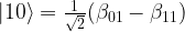
The first step in the algorithm is to prepare an entangled state

$|\beta_{00}^{AB} \rangle = \frac{1}{\sqrt{2}} \big[ |0\rangle _A |0 \rangle _B+ |1\rangle_A |1 \rangle_B) \big]$

Here the upper index at $\beta$ indicates the two qubits in which the Bell state vector lives. This is the common state mentioned above, and it can obviously be prepared upfront, without having the state $|\psi \rangle_C$ . Bob and Alice could even prepare an entire repository of such states, ready for being used when the actual transmission should take place.

Now let us look at the state of the combined system consisting of all three qubits.

$|\beta_{00}^{AB} \rangle |\psi\rangle_C = \frac{1}{\sqrt{2}} \big[ a |000 \rangle + a |110 \rangle + b |001\rangle + b |111 \rangle \big]$

For a reason that will become clear in a second, we will now adapt the tensor product order and choose the new order A-C-B. Then our state is (simply swap the last two qubits)

$\frac{1}{\sqrt{2}} \big[ a |000 \rangle + a |101 \rangle + b |010\rangle + b |111 \rangle \big]$

Now instead of using the computational basis for our three-qubit system, we could as well use the basis that is given by the Bell basis of the qubits A and C and the computational basis of B, i.e. $|\beta^{AC}_{ij} \rangle |k\rangle$ . Using the table above, we can express our state in this basis. This will give us four terms that contain a and four terms that contain b. The terms that contain a are

$\frac{a}{2} \big[ |\beta^{AC}_{00}\rangle |0 \rangle + |\beta^{AC}_{10}\rangle |0 \rangle + |\beta^{AC}_{01}\rangle |1 \rangle - |\beta^{AC}_{11} \rangle |1 \rangle \big]$

and the terms that contain b are

$\frac{b}{2} \big[ |\beta^{AC}_{01}\rangle |0 \rangle + |\beta^{AC}_{11}\rangle |0 \rangle + |\beta^{AC}_{00}\rangle |1 \rangle - |\beta^{AC}_{10} \rangle |1 \rangle \big]$

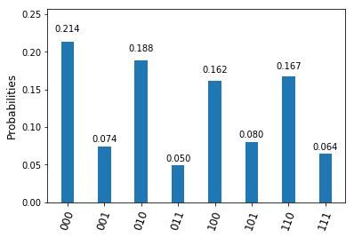
So far we have not done anything to our state, we have simply re-written the state as an expansion into a different basis. Now Alice conducts a measurement – but she measures A and C in the Bell basis. This will project the state onto one of the basis vectors $|\beta_{ij}^{AC}\rangle$ . Thus there are four different possible outcomes of this measurement, which we can read off from the expansion in terms of the Bell basis above.

Measurement	State of qubit B
$\beta_{00}$	$a\|0\rangle + b\|1\rangle = \|\psi \rangle$
$\beta_{01}$	$a\|1\rangle + b\|0\rangle = X\|\psi \rangle$
$\beta_{10}$	$a\|0\rangle - b\|1\rangle = Z\|\psi \rangle$
$\beta_{11}$	$b\|0\rangle - a\|1\rangle = -XZ\|\psi \rangle$

Now Alice sends the outcome of the measurement to Bob using the classical channel. The table above shows that the state in Bob’s qubit B is now the result of a unitary transformation which depends only on the measurement outcome. Thus if Bob receives the measurement outcomes (two bits), he can do a lookup on the table above and apply the inverse transformation on his qubit. If, for instance, he receives the measurement outcome 01, he can apply a Pauli X gate to his qubit and then knows that the state in this qubit will be identical to the original state $|\psi \rangle$ . The teleportation process is complete.

Implementing teleportation as a circuit

Let us now build a circuit that models the teleportation procedure. The first part that we need is a circuit that creates a Bell state (or, more generally, transforms the elements of the computational basis into the Bell basis). This is achieved by the circuit below (which again uses the Qiskit convention that the most significant qubit q₁ is the leftmost one in the tensor product).

It is obvious how this circuit can be reversed – as both individual gates used are there own inverse, we simply need to reverse their order to obtain a circuit that maps the Bell basis to the computational basis.

Let us now see how the overall teleportation circuit looks like. Here is the circuit (drawn with Qiskit).

Let us see how this relates to the above description. First, the role of the qubits is, from the top to the bottom

C = q[2]
A = q[1]
B = q[0]

The first two gates (the Hadamard and the CNOT gate) act on qubits A and B and create the Bell basis vector $\beta_{00}$ from the initial state. This state is the shared entangled state that Alice and Bob prepare upfront.

The next section of the circuit operates on the qubits A and C and realizes the measurement in the Bell basis. We first use a combination of another CNOT gate and another Hadamard gate to map the Bell basis to the computational basis and then perform a measurement – these steps are equivalent to doing a measurement in the Bell basis directly.

Finally, we have a controlled X gate and a controlled Z gate. As described above, these gates apply the conditional corrections to Bob’s state in qubit B that depend on the outcome of the measurement. As a result, the state of qubit B will be the same as the initial state of qubit C.

How can we test this circuit? One approach could be to add a pre-processing part and a post-processing part to our teleportation circuit. The pre-processing gate acts with one or more gates on qubit C to put this qubit into a defined state. We then apply the teleportation circuit. Finally, we apply a post-processing circuit, namely the inverse sequence of gates to the “target” of the teleportation, i.e. to qubit B. If the teleportation works, the pre- and post-steps act on the same logical state and therefore cancel each other. Thus the final result in qubit B will be the initial state of qubit C, i.e. $|0 \rangle$ . 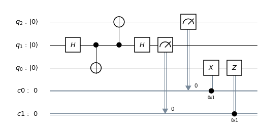Therefore, a measurement of this qubit will always yield zero. Thus our final test circuit looks as follows.

When we run this on a simulator, the result will be as expected – the value in the classical register c2 after the measurement will always be zero. I have not been able to test this on real hardware as the IBM device does not (yet?) support classical conditional gates, but the result is predictable – we would probably get the same output with some noise. If you want to play with the circuits yourself, you can, as always, find the code in my GitHub repository.

So this is quantum teleportation – not quite as mysterious as the name suggests. In particular, we do not magically teleport particles and actual matter, but simply quantum information, based on a clever split of the information contained in an unknown state into a classical part, transmitted in two classical bit, and a quantum part that we can prepare upfront. We also do not violate special relativity – to complete the process, we depend on the measurement outcomes that are transmitted via a classical channel and therefore not faster than the speed of light. It is also important to note that quantum teleportation does also not violate the “no-cloning”-principle – the measurements let the original state collapse and therefore we do not end up with two copies of the same state.

Quantum teleportation has already been demonstrated in reality several times. The first experimental verification was published in [3] in 1997. Since then, the distance between the involved parties “Alice” and “Bob” has been gradually increased. In 2017, a chinese team reported a teleportation of a single qubit between a ground observatory to a low-Earth-orbit satellite (see [4]).

The term quantum teleportation is also used in the context of quantum error correction for a circuit that uses a measurement on an entangled state to bring one of the involved qubits into a specific state. When using a surface code, for instance, this technique – also called gate teleportation – is used to implement the T gate on the level of logical qubits. We refer to [5] for a more detailed discussion of this pattern.

References

1. M. Nielsen, I. Chuang, Quantum Computation and Quantum Information, Cambridge University Press, Cambridge 2010
2. C.H. Bennett, G. Brassard, C. Crepeau, R. Jozsa, A Peres, W.K. Wootter, Teleporting an Unknown Quantum State via Dual Classical and EPR Channels, Phys. Rev. Lett. 70, March 1993
3. D. Bouwmeester, Jian-Wei Pan, K. Mattle, M. Eibl, H. Weinfurter, A. Zeilinger, Experimental quantum teleportation, Nature Vol. 390, Dec. 1997
4. Ji-Gang Ren et. al., Ground-to-satellite quantum teleportation, Nature Vol. 549, September 2017
5. D. Gottesman, I. L. Chuang, Quantum Teleportation is a Universal Computational Primitive, arXiv:quant-ph/9908010

Kubernetes services and load balancers

In my previous post, we have seen how we can use Kubernetes deployment objects to bring up a given number of pods running our Docker images in a cluster. However, most of the time, a pod by itself will not be able to operate – we need to connect it with other pods and the rest of the world, in other words we need to think about networking in Kubernetes.

To try this out, let us assume that you have a cluster up and running and that you have submitted a deployment of two httpd instances in the cluster. To easily get to this point, you can use the scripts in my GitHub repository as follows. These scripts will also open two ssh connections, one to each of the EC2 instances which are part of the cluster (this assumes that you are using a PEM file called eksNodeKey.pem as I have done it in my examples, if not you will have to adjust the script up.sh accordingly).

# Clone repository
$ git clone https://github.com/christianb93/Kubernetes.git
$ cd Kubernetes/cluster
# Bring up cluster and two EC2 nodes
$ chmod 700 up.sh
$ ./up.sh
# Bring down nginx controller
$ kubectl delete svc ingress-nginx -n ingress-nginx
# Deploy two instances of the httpd
$ kubectl apply -f ../pods/deployment.yaml

Be patient, the creation of the cluster will take roughly 15 minutes, so time to get a cup of coffee. Note that we delete an object – the nginx ingress controller service – that my scripts generate and that we will use in a later post, but which blur the picture for today.

Now let us inspect our cluster and try out a few things. First, let us get the running pods.

$ kubectl get pods -o wide

This should give you two pods, both running an instance of the httpd. Typically, Kubernetes will distribute these two pods over two different nodes in the cluster. Each pod has an IP address called the pod IP address which is displayed in the column IP of the output. This is the IP address under which the pod is reachable from other pods in the cluster.

To verify this, let us attach to one of the pods and run curl to access the httpd running in the other pod. In my case, the first pod has IP address 192.168.232.210. We will attach to the second pod and verify that this address is reachable from there. To get a shell in the pod, we can use the kubectl exec command which executes code in a pod. The following commands extract the id of the second pod, opens a shell in this pod, installs curl and talks to the httpd in the first pod. Of course, you will have to replace the IP address of the first pod – 192.168.232.210 – with whatever your output gives you.

$ name=$(kubectl get pods --output json | \
             jq -r ".items[1].metadata.name")
$ kubectl exec -it $name "/bin/bash"
bash-4.4# apk add curl
bash-4.4# curl 192.168.232.210
<h1>It works!</h1>

Nice. So we can reach a port on pod A from any other pod in the cluster. This is what is called the flat networking model in Kubernetes. In this model, each pod has a separate IP address. All containers in the pod share this IP address and one IP namespace. Every pod IP address is reachable from any other pod in the cluster without a need to set up a gateway or NAT. Coming back to the comparison of a pod with a logical host, this corresponds to a topology where all logical hosts are connected to the same IP network.

In addition, Kubernetes assumes that every node can reach every pod as well. You can easily confirm this – if you log into the node (not the pod!) on which the second pod is running and use curl from there, directed to the IP address of the first pod, you will get the same result.

Now Kubernetes is designed to run on a variety of platforms – locally, on a bare metal cluster, on GCP, AWS or Azure and so forth. Therefore, Kubernetes itself does not implement those rules, but leaves that to the underlying platform. To make this work, Kubernetes uses an interface called CNI (container networking interface) to talk to a plugin that is responsible for executing the platform specific part of the network configuration. On EKS, the AWS CNI plugin is used. We will get into the details in a later post, but for the time being simply assume that this works (and it does).

So now we can reach every pod from every other pod. This is nice, but there is an issue – a pod is volatile. An application which is composed of several microservices needs to be prepared for the event that a pod goes down and is brought up again, be it due to a failure or simply due to the fact that an auto-scaler tries to empty a node. If, however, a pod is restarted, it will typically receive a different IP address.

Suppose, for instance, you had a REST service that you want to expose within your cluster. You use a deployment to start three pods running the REST service, but which IP address should another service in the cluster use to access it? You cannot rely on the IP address of individual pods to be stable. What we need is a stable IP address which is reachable by all pods and which routes traffic to one instance of this REST service – a bit like a cluster-internal load balancer.

Fortunately, Kubernetes services come to the rescue. A service is a Kubernetes object that has a stable IP address and is associated with a set of pods. When traffic is received which is directed to the service IP address, the service will select one of the pods (at random) and forward the traffic to it. Thus a service is a decoupling layer between the instable pod IP addresses and the rst of the cluster or the outer world. We will later see that behind the scenes, a service is not a process running somewhere, but essentially a set of smart NAT and routing rules.

This sounds a bit abstract, so let us bring up a service. As usual, a service object is described in a manifest file.

apiVersion: v1
kind: Service
metadata:
  name: alpine-service
spec:
  selector:
    app: alpine
  ports:
  - protocol: TCP
    port: 8080
    targetPort: 80

Let us call this file service.yaml (if you have cloned my repository, you already have a copy of this in the directory network). As usual, this manifest file has a header part and a specification section. The specification section contains a selector and a list of ports. Let us look at each of those in turn.

The selector plays a role similar to the selector in a deployment. It defines a set of pods that are assumed to be reachable via the service. In our case, we use the same selector as in the deployment, so that our service will send traffic to all pods brought up by this deployment.

The ports section defines the ports on which the service is listening and the ports to which traffic is routed. In our case, the service will listen for TCP traffic on port 8080, and will forward this traffic to port 80 on the associated pods (as specified by the selector). We could omit the targetPort field, in this case the target port would be equal to the port. We could also specify more than one combination of port and target port and we could use names instead of numbers for the ports – refer to the documentation for a full description of all configuration options.

Let us try this. Let us apply this manifest file and use kubectl get svc to list all known services.

$ kubectl apply -f service.yaml
$ kubectl get svc

You should now see a new service in the output, called alpine-service. Similar to a pod, this service has a cluster IP address assigned to it, and a port number (8080). In my case, this cluster IP address is 10.100.234.120. We can now again get a shell in one of the pods and try to curl that address

$ name=$(kubectl get pods --output json | \
             jq -r ".items[1].metadata.name")
$ kubectl exec -it $name "/bin/bash"
bash-4.4# apk add curl # might not be needed 
bash-4.4# curl 10.100.234.120:8080
<h1>It works!</h1>

If you are lucky and your container did not go down in the meantime, curl will already be installed and you can skip the apk add curl. So this works, we can actually reach the service from within our cluster. Note that we now have to use port 8080, as our service is listening on this port, not on port 80.

You might ask how we can get the IP address of the service in real world? Well, fortunately Kubernetes does a bit more – it adds a DNS record for the service! So within the pod, the following will work

bash-4.4# curl alpine-service:8080
<h1>It works!</h1>

So once you have the service name, you can reach the httpd from every pod within the cluster.

Connecting to services using port forwarding

Having a service which is reachable within a cluster is nice, but what options do we have to reach a cluster from the outside world? For a quick and dirty test, maybe the easiest way is using the kubectl port forwarding feature. This command allows you to forward traffic from a local port on your development machine to a port in the cluster which can be a service, but also a pod. In our case, let us forward traffic from the local port 5000 to port 8080 of our service (which is hooked up to port 80 on our pods).

$ kubectl port-forward service/alpine-service 5000:8080

This will start an instance of kubectl which will bind to port 5000 on your local machine (127.0.0.1). You can now connect to this port, and behind the scenes, kubectl will tunnel the traffic through the Kubernetes master node into the cluster (you need to run this in a second terminal, as the kubectl process just started is still blocking your terminal).

$ curl localhost:5000
<h1>It works!</h1>

A similar forwarding can be realized using kubectl proxy, which is designed to give you access to the Kubernetes API from your local machine, but can also be used to access services.

Connect to a service using host ports

Forwarding is easy and a quick solution, but most likely not what you want to do in a production setup. What other options do we have?

One approach is to use host ports. Essentially, a host port is a port on a node that Kubernetes will wire up with the cluster IP address of a service. Assuming that you can reach the host from the outside world, you can then use the public IP address of the host to connect to a service.

To create a host port, we have to modify our manifest file slightly by adding a host port specification.

apiVersion: v1
kind: Service
metadata:
  name: alpine-service
spec:
  selector:
    app: alpine
  ports:
  - protocol: TCP
    port: 8080
    targetPort: 80
  type: NodePort

Note the additional line at the bottom of the file which instructs Kubernetes to open a node port. Assuming that this file is called nodePortService.yaml, we can again use kubectl to bring down our existing service and add the node port service.

$ kubectl delete svc alpine-service
$ kubectl apply -f nodePortService.yaml
$ kubectl get svc

We see that Kubernetes has brought up our service, but this time, we see two ports in the line describing our service. The second port (32226 in my case) is the port that Kubernetes has opened on each node. Traffic to this port will be forwarded to the service IP address and port. To try this out, you can use the following commands to get the external IP address of the first node, adapt the AWS security group such that traffic to this node is allowed from your workstation, determine the node port and curl it. If your cluster is not called myCluster, replace every occurrence of myCluster with the name of your cluster.

$ nodePort=$(kubectl get svc alpine-service --output json | jq ".spec.ports[0].nodePort")
$ IP=$(aws ec2 describe-instances --filters Name=tag-key,Values=kubernetes.io/cluster/myCluster Name=instance-state-name,Values=running --output text --query Reservations[0].Instances[0].PublicIpAddress)
$ SEC_GROUP_ID=$(aws ec2 describe-instances --filters Name=tag-key,Values=kubernetes.io/cluster/myCluster Name=instance-state-name,Values=running --output text --query Reservations[0].Instances[0].SecurityGroups[0].GroupId)
$ myIP=$(wget -q -O- https://ipecho.net/plain)
$ aws ec2 authorize-security-group-ingress --group-id $SEC_GROUP_ID --port $nodePort --protocol tcp --cidr "$myIP/32"
$ curl $IP:$nodePort
<h1>It works!</h1>

Connecting to a service using a load balancer

A node port will allow you to connect to a service using the public IP of a node. However, if you do this, this node will be a single point of failure. For a HA setup, you would typically choose a different options – load balancers.

Load balancers are not managed directly by Kubernetes. Instead, Kubernetes will ask the underlying cloud provider to create a load balancer for you which is then connected to the service – so there might be additional charges. Creating a service exposed via a load balancer is easy – just change the type field in the manifest file to LoadBalancer

apiVersion: v1
kind: Service
metadata:
  name: alpine-service
spec:
  selector:
    app: alpine
  ports:
  - protocol: TCP
    port: 8080
    targetPort: 80
  type: LoadBalancer

After applying this manifest file, it takes a few seconds for the load balancer to be created. Once this has been done, you can find the external DNS name of the load balancer (which AWS will create for you) in the column EXTERNAL-IP of the output of kubectl get svc. Let us extract this name and curl it. This time, we use the jsonpath option of the kubectl command instead of jq.

$ host=$(kubectl get svc alpine-service --output  \
         jsonpath="{.status.loadBalancer.ingress[0].hostname}")
$ curl $host:8080
<h1>It works!</h1>

If you get a “couldn not resolve hostname” error, it might be that the DNS entry has not yet propagated through the infrastructure, this might take a few minutes.

What has happened? Behind the scenes, AWS has created an elastic load balancer (ELB) for you. Let us describe this load balancer.

$ aws elb describe-load-balancers --output json
{
    "LoadBalancerDescriptions": [
        {
            "Policies": {
                "OtherPolicies": [],
                "LBCookieStickinessPolicies": [],
                "AppCookieStickinessPolicies": []
            },
            "AvailabilityZones": [
                "eu-central-1a",
                "eu-central-1c",
                "eu-central-1b"
            ],
            "CanonicalHostedZoneName": "ad76890d448a411e99b2e06fc74c8c6e-2099085292.eu-central-1.elb.amazonaws.com",
            "Subnets": [
                "subnet-06088e09ce07546b9",
                "subnet-0d88f92baecced563",
                "subnet-0e4a8fd662faadab6"
            ],
            "CreatedTime": "2019-03-17T11:07:41.580Z",
            "SecurityGroups": [
                "sg-055b253a63c7aba0a"
            ],
            "Scheme": "internet-facing",
            "VPCId": "vpc-060469b2a294de8bd",
            "LoadBalancerName": "ad76890d448a411e99b2e06fc74c8c6e",
            "HealthCheck": {
                "UnhealthyThreshold": 6,
                "Interval": 10,
                "Target": "TCP:30829",
                "HealthyThreshold": 2,
                "Timeout": 5
            },
            "BackendServerDescriptions": [],
            "Instances": [
                {
                    "InstanceId": "i-0cf7439fd8eb65858"
                },
                {
                    "InstanceId": "i-0fda48856428b9a24"
                }
            ],
            "SourceSecurityGroup": {
                "GroupName": "k8s-elb-ad76890d448a411e99b2e06fc74c8c6e",
                "OwnerAlias": "979256113747"
            },
            "DNSName": "ad76890d448a411e99b2e06fc74c8c6e-2099085292.eu-central-1.elb.amazonaws.com",
            "ListenerDescriptions": [
                {
                    "PolicyNames": [],
                    "Listener": {
                        "InstancePort": 30829,
                        "LoadBalancerPort": 8080,
                        "Protocol": "TCP",
                        "InstanceProtocol": "TCP"
                    }
                }
            ],
            "CanonicalHostedZoneNameID": "Z215JYRZR1TBD5"
        }
    ]
}

This is a long output, let us see what this tells us. First, there is a list of instances, which are the instances of the nodes in your cluster. Then, there is the block ListenerDescriptions. This block specificies, among other things, the load balancer port (8080 in our case, this is the port that the load balancer exposes) and the instance port (30829). You will note that these are also the ports that kubectl get svc will give you. So the load balancer will send incoming traffic on port 8080 to port 30829 of one of the instances. This in turn is a host port as discussed before, and therefore will be connected to our service. Thus, even though technically not fully correct, the following picture emerges (technically, a service is not a process, but a collection of iptables rules on each node, which we will look at in more detail in a later post).

Using load balancers, however, has a couple of disadvantages, the most obvious one being that each load balancer comes with a cost. If you have an application that exposes tens or even hundreds of services, you clearly do not want to fire up a load balancer for each of them. This is where an ingress comes into play, which can distribute incoming HTTP(S) traffic across various services and which we will study in one of the next posts.

There is one important point when working with load balancer services – do not forget to delete the service when you are done! Otherwise, the load balancer will continue to run and create charges, even if it is not used. So delete all services before shutting down your cluster and if in doubt, use aws elb describe-load-balancers to check for orphaned load balancers.

Creating services in Python

Let us close this post by looking into how services can be provisioned in Python. First, we need to create a service object and populate its metadata. This is done using the following code snippet.

service = client.V1Service()
service.api_version = "v1"
service.kind = "Service"
metadata = client.V1ObjectMeta(name="alpine-service")
service.metadata = metadata
service.type="LoadBalancer"

Now we assemble the service specification and attach it to the service object.

spec = client.V1ServiceSpec()
selector = {"app": "alpine"}
spec.selector = selector
spec.type="LoadBalancer"
port = client.V1ServicePort(
              port = 8080, 
              protocol = "TCP", 
              target_port = 80 )
spec.ports = [port]
service.spec = spec

Finally, we authenticate, create an API endpoint and submit the creation request.

config.load_kube_config()
api = client.CoreV1Api()
api.create_namespaced_service(
         namespace="default", 
         body=service)

If you have cloned my GitHub repository, you will find a script network/create_service.py that contains the full code for this and that you can run to try this out (do not forget to delete the existing service before running this).

Kubernetes 101 – creating pods and deployments

In the last posts, we have seen how we can set up a Kubernetes cluster on Amazons EKS platform and spin up our first nodes. Today, we will create our first workloads and see pods and deployments in action.

Creating pods

We have already introduces pods in an earlier post as the smallest units that Kubernetes manages. To create pods, there are several options. First, we can use the kubectl command line tool and simply pass the description of the pod as arguments. Second, we can use a so-called manifest file which contains the specification of the pod, which has the obvious advantage that this file can be reused, put under version control, developed and tested, according to the ideas of the “Infrastructure as a code” approach. A manifest file can either be provided in JSON format or using the YAML markup language. And of course, we can again use the Kubernetes API directly, for instance by programming against the Python API.

In this post, we will demonstrate how to create pods using manifest file in YAML format and Python scripts. We start with a YAML file which looks as follows.

apiVersion: v1
kind: Pod
metadata:
  name: naked-pod-demo
  namespace: default
spec:
  containers:
  - name: naked-pod-demo-ctr
    image: nginx

Let us go through this file step by step to understand what it means. First, this is a YAML file, and YAML is essentially a format for specifying key-value pairs. Our first key is apiVersion, with value v1. This is the first line in all manifest files and simply specifies the API version that we will use.

The next key – kind – specifies the type of Kubernetes resource that we want to access, in this case a pod. The next key is metadata. The value of this key is a dictionary that again has two keys – name and namespace. The name is the name that our pod will have. The namespace key specifies the namespace in which the pod will start (namespaces are a way to segment Kubernetes resources and are a topic for a future post, for the time being we will simply use the so-called default namespace).

The next key – spec now contains the actual specification of the pod. This is where we tell Kubernetes what our pod should be running. Remember that a pod can contain one or more application containers. Therefore there is a key containers, which, as a value, has a list of containers. Each container has a name and further attributes.

In our case, we create one container and specify that the image should be nginx. At this point, we can specify every image that we could also specify if we did a docker run locally. In this case, Kubernetes will pull the nginx image from the default docker registry and run it.

So let us now trigger the creation of a pod by passing this specification to kubectl. To do this, we use the following command (assuming that you have saved the file as naked_pod.yaml, the reason for this naming will become clear later).

kubectl apply -f naked_pod.yaml

After a few seconds, Kubernetes should have had enough time to start up the container, so let us use kubectl to check whether the node has been created.

$ kubectl get pods 
NAME             READY   STATUS    RESTARTS   AGE
naked-pod-demo   1/1     Running   0          38s

Nice. Let us take a closer look at this pod. If you run kubectl get pods -o wide, kubectl will give you a bit more information on the pod, including the name of the node on which the pod is running. So let us SSH into this node. To easily log into one of your nodes (the first node in this case, change Node to 1 to log into the second node), you can use the following sequence of commands. This will open the SSH port for all instances in the cluster for incoming connections from the your current IP address. Note that we use the cluster name as a filter, so you might need to replace myCluster in the commands below by the name of your cluster.

$ Node=0
$ IP=$(aws ec2 describe-instances --output text --filters Name=tag-key,Values=kubernetes.io/cluster/myCluster Name=instance-state-name,Values=running --query Reservations[$Node].Instances[0].PublicIpAddress)
$ SEC_GROUP_ID=$(aws ec2 describe-instances  --output text --filters Name=tag-key,Values=kubernetes.io/cluster/myCluster Name=instance-state-name,Values=running --query Reservations[0].Instances[0].SecurityGroups[0].GroupId)
$ myIP=$(wget -q -O- https://ipecho.net/plain)
$ aws ec2 authorize-security-group-ingress --group-id $SEC_GROUP_ID --port 22 --protocol tcp --cidr $myIP/32
$ ssh -i ~/eksNodeKey.pem ec2-user@$IP

Use this – or your favorite method (if you use my script up.sh to start the cluster, it will already open ssh connections to both nodes for you) – to log into the node on which the pod has been scheduled by Kubernetes and execute a docker ps there. You should see that, among some management containers that Kubernetes brings up, a container running nginx appears.

Now let us try a few things. First, apply the YAML file once more. This will not bring up a second pod. Instead, Kubernetes realizes that a pod with this name is already running and tells you that no change has been applied. This makes sense – in general, a manifest file specifies a target state, and we are already in the target state, so there is no need for action.

Now, on the EKS worker node on which the pod is running, use docker kill to actually stop the container. Then wait for a few seconds and do a docker ps again. Surprisingly, you will see the container again, but with a different container ID. What happened?

The answer is hidden in the logfiles of the component of Kubernetes that controls a single node – the kubelet. On the node, the kubelet is started using systemctl (you might want to verify this in the AWS provided bootstrap.sh script). So to access its logs, we need

$ journalctl -u kubelet

Close to the end of the logfile, you should see a line stating that … container … is dead, but RestartPolicy says that we should restart it. In fact, the kubelet constantly monitors the running containers and looks for deviations from the target state. The restart policy is a piece of the specification of a pod that tells the kubelet how to handle the case that a container has died. This might be perfectly fine (for batch jobs), but the default restart policy is Always, so the the kubelet will restart our container.

This is nice, but now let us simulate a more drastic event – the node dies. So on the AWS console, locate the node on which the pod is running and terminate the pod.

After a few seconds, you will see that a new node is created, thanks to the AWS auto-scaling group that controls our nodes. However, if you check the status of the pods using kubectl get pods, you will see that Kubernetes did not reschedule the pod on a different node, nor does it restart the pod once the replacement node is up and running again. So Kubernetes takes care (via the kubelet) of the containers that belong to a pod on a per-node level, but not on a per-cluster level.

In productions, this is of course typically not what you want – instead, it would be nice if Kubernetes could monitor the pods for you and restart them automatically in case of failure. This is what a deployment does.

Replica sets and deployments

A deployment is an example for a more general concept in Kubernetes – controllers. Basically, this is a component that constantly monitors the cluster state and makes changes if needed to get back into the target state. One thing that a deployment does is to automatically bring up a certain number of instances called replicas of a Docker image and distribute the resulting pods across the cluster. Once the pods are running, the deployment controller will monitor them and take action of the number of pods running deviates from the desired number of pods. As an example, let us consider the following manifest file.

apiVersion: apps/v1
kind: Deployment
metadata:
  name: alpine
spec:
  selector:
    matchLabels:
      app: alpine
  replicas: 2
  template:
    metadata:
      labels:
        app: alpine
    spec:
      containers:
        - name: alpine-ctr
          image: httpd:alpine

The first line is specifying the API version as usual (though we need to use a different value for the API version, the additional apps is due to the fact that the Deployment API is part of the API group apps). The second line designates the object that we want to create as a deployment. We then again have a name which is part of the metadata, followed by the actual specification of the deployment.

The first part of this specification is the selector. To understands its role, recall that a deployment is supposed to make sure that a specified number of pods of a given type are running. Now, the term “of a given type” has to be made precise, and this is what the selector is being used for. All pods which are created by our deployment will have a label with key “app” and value “alpine”. The selector field specifies that all pods with that label are to be considered as pods controlled by the deployment, and our controller will make sure that there are always exactly two pods with this label.

The second part of the specification is the template that the deployment uses to create the pods controlled by this deployment. This looks very much like the definition of a pod as we have seen it earlier. However, the label that is specified here of course needs to match the label in the selector field (kubectl will actually warn you if this is not the case).

Let us now delete our existing pod, run this deployment and see what is happening. Save the manifest file as deployment.yaml, apply it and then list the running nodes.

$ kubectl delete -f naked_pod.yaml
$ kubectl apply -f deployment.yaml
deployment.apps/alpine created
$ kubectl get pods
NAME                      READY   STATUS    RESTARTS   AGE
alpine-8469fc798f-rq92t   1/1     Running   0          21s
alpine-8469fc798f-wmsqc   1/1     Running   0          21s

So two pods have been created and scheduled to nodes of our cluster. To inspect the container further, let us ask kubectl to provide all details as JSON and use the wonderful jq to process the output and extract the container information from it (you might need to install jq to run this).

$ kubectl get pods --output json | jq ".items[0].spec.containers[0].image"
"httpd:alpine"

So we see that the pods and the containers have been created according to our specification and run the httpd:alpine docker image.

Let us now repeat our experiment from before and stop one of the node. To do this, we first extract the instance ID of the first instance using the AWS CLI and then use the AWS CLI once more to stop this instances.

$ instanceId=$(aws ec2 describe-instances --output text --filters Name=tag-key,Values=kubernetes.io/cluster/myCluster Name=instance-state-name,Values=running --query Reservations[0].Instances[0].InstanceId)
$ aws ec2 terminate-instances --instance-ids $instanceId

After some time, Kubernetes will find that the instance has died, and if you run a kubectl get nodes, you will find that the node has disappeared. If you now run kubectl get nodes -o wide, however, you will still find two pods, but now both are running on the remaining node. So the deployment controller has replaced the pod that went down with our node by a new pod on the remaining node. This behaviour is in fact not realized by the deployment, but by the underlying ReplicaSet. We could also create a replica set directly, but a deployment offers some additional features, like the possibility to run a rolling upgrade automatically.

Creating deployments in Python

Having discussed how to create a deployment from a YAML file, let us again do the same thing in Python. The easiest approach is to walk our way upwards through the YAML file. After the usual preparations (imports, loading the configuration), we therefore start with the specification of the container.

import client
container = client.V1Container(
              name="alpine-ctr",
              image="httpd:alpine")

This is similar to our YAML file – in each pod, we want to run a container with the httpd:alpine image. Having the container object, we can now create the template section.

template = client.V1PodTemplateSpec(
        metadata=client.V1ObjectMeta(
                   labels={"app": "alpine"}),
        spec=client.V1PodSpec(containers=[container]))

Again, note the label that we will use later to select the pods that our deployment controller is supposed to watch. Now we put the template into the specification part of our controller.

selector = client.V1LabelSelector(
              match_labels={"app" : "alpine"})
spec = client.V1DeploymentSpec(
        replicas=2,
        template=template, 
        selector=selector)

And finally, we can create the actual deployment object and ask Kubernetes to apply it – the complete Python script is available for download here).

deployment = client.V1Deployment(
       api_version="apps/v1",
       kind="Deployment",
       metadata=client.V1ObjectMeta(name="alpine"),
       spec=spec)

apps.create_namespaced_deployment(
              namespace="default", body=deployment)

This completes our post for today. We now know how to create pods and deployments to run Docker images in our cluster. In the next few posts, we will look at networking in Kubernetes – services, load balancers, ingress and all that.

Python up an EKS cluster – part II

In the last post, we have seen how Python can be used to control the generation of an EKS cluster. However, an EKS cluster without any worker nodes – and hence without the ability to start pods and services – is of very limited use. Today, we therefore take a look at the process of adding worker nodes.

Again, we roughly follow the choreography of Amazons Getting started with EKS guide, but instead of going through the individual steps using the console first, we start using the API and the Python SDK right away.

This description assumes that you have started an EKS cluster as described in my last post. If not, you can do this by running the create_cluster Python script that executes all necessary steps.

Essentially, we will do two things. First, we will create an AWS Auto-Scaling group that we will use to manage our worker nodes. This can be done using the AWS API and the Python SDK. Part of this setup will be a new role, that, in a second step, we need to make known to Kubernetes so that our nodes can join the cluster. This will be done using the Kubernetes API. Let us now look at each of these steps in turn.

Creating an auto-scaling group

An auto-scaling group is essentially a group of EC2 instances that are combined into one management unit. When you set up an auto-scaling group, you specify a scaling policy and AWS will apply that policy to make sure that a certain number of instances is automatically running in your group. If the number of instances drops below a certain value, or if the load increases (depending on the policy), then AWS will automatically spin up new instances for you.

We will use AWS CloudFormation to set up the auto-scaling group, using the template referenced in the “Getting started” guide. This is not an introduction into CloudFormation, but it is instructive to look at this template, stored at this URL.

If you look at this file, you will recognize a few key elements. First, there are parameters whose values we will have to provide when we use the template. These parameters are

A unique name for the node group
The name of an SSH key pair that we will later use to log into our nodes. I recommend to create a separate key pair for this, and I will assume that you have done this and that this key pair is called eksNodeKey
An instance type that AWS will use to spin up nodes
The ID of an AMI image that will be used to spin up the nodes. In this tutorial, we will use Kubernetes v1.11 and the specific AWS provided AMIs which are listed in the Getting started guide. I work in the region eu-frankfurt-1, and will therefore use the AMI ID ami-032ed5525d4df2de3
The minimum, maximum and desired size of the auto-scaling group. We will use one for the minimum size, two for the desired size and three for the maximum size, so that our cluster will come up with two nodes initially
The size of the volume attached to each node – we will not provide a value for this and stick to the default (20 GB at the time of writing)
In addition, we will have to supply the VPC, the subnets and the security group that we used before

In addition to the parameters, the CloudFormation template contains a list of resources that will be created. We see that in addition to several security groups and the auto scaling group, a IAM role called the node instance role and a corresponding instance profile is created. This is the role that the nodes will assume to interact with the Kubernetes master, and behind the scenes, the AWS IAM authenticator will be used to map this IAM role to a Kubernetes user, so that the nodes can authenticate themselves against the Kubernetes API. This requires some configuration, more precisely a mapping between IAM roles and Kubernetes users, which we will set up in our second steps in the next section.

So how do we apply this cloud formation template? Again, the AWS API comes to the rescue. It provides an API endpoint (client) for CloudFormation which has a method create_stack. This method expects a Python data structure that contains the parameters that we want to use, plus the URL of the cloud formation template. It will then take the template, apply the parameters, and create the resources defined in the template.

Building the parameter structure is easy, assuming that you have already stored all configuration data in Python variables (we can use the same method as in the last post to retrieve cluster data like the VPC ID). The only tricky part is the list of subnets. In CloudFormation, a parameter value that is a list needs to be passed as a comma separated list, not as a JSON list (it took me some failed attempts to figure out this one). Hence we need to convert our list of subnets into CSV format. The code snippet to set up the parameter map then looks as follows.

params = [
  {'ParameterKey' : 'KeyName' , 
   'ParameterValue' : sshKeyPair },
  {'ParameterKey' : 'NodeImageId' , 
   'ParameterValue' : amiId },
  {'ParameterKey' : 'NodeInstanceType' , 
   'ParameterValue' : instanceType },
  {'ParameterKey' : 'NodeAutoScalingGroupMinSize' , 
   'ParameterValue' : '1' },
  {'ParameterKey' : 'NodeAutoScalingGroupMaxSize' , 
   'ParameterValue' : '3' },
  {'ParameterKey' : 'NodeAutoScalingGroupDesiredCapacity' , 
   'ParameterValue' : '2' },
  {'ParameterKey' : 'ClusterName' , 
   'ParameterValue' : clusterName },
  {'ParameterKey' : 'NodeGroupName' , 
   'ParameterValue' : nodeGroupName },
  {'ParameterKey' : 'ClusterControlPlaneSecurityGroup' , 
   'ParameterValue' : secGroupId },
  {'ParameterKey' : 'VpcId' , 
   'ParameterValue' : vpcId },
  {'ParameterKey' : 'Subnets' , 
   'ParameterValue' : ",".join(subnets) },
]

Some of the resources created by the template are IAM resources, and therefore we need to confirm explicitly that we allow for this. To do this, we need to specify a specific capability when calling the API. With that, our call now looks as follows.

cloudFormation = boto3.client('cloudformation')
cloudFormation.create_stack(
  StackName = stackName, 
  TemplateURL = templateURL,
  Parameters = params,
  Capabilities = ['CAPABILITY_IAM'])

Here the template URL is the location of the CloudFormation template provided above, and stack name is some unique name that we use for our stack (it is advisable to include the cluster name, so that you can create and run more than one cluster in parallel).

When you run this command, several things will happen, and it is instructive to take a look at the EC2 console and the CloudFormation console while the setup is in progress. First, you will find that a new stack appears on the CloudFormation console, being in status “In Creation”.

Second, the EC2 console will display – after a few seconds – a newly created auto scaling group, with the parameters specified in the template, and a few additional security groups.

And when you list your instances, you will find that AWS will spin up two instances of the specified type. These instances will come up as usual and are ordinary EC2 instances.

Remember that we specified a key pair when we created the auto-scaling group? Hopefully, you did save the PEM file – if yes, you can now SSH into your nodes. For that purpose, you will have to modify the security group of the nodes and open the SSH port for inbound traffic from your own network. Once this has been done, you can simply use an ordinary SSH command to connect to your machines.

$ ssh -i eksNodeKey.pem ec2-user@18.197.140.230

where of course you need to replace 18.197.140.230 with whatever public IP address the instance has. You can now inspect the node, for instance doing docker ps to see which docker containers are already running on the node, and you can use ps ax to see which processes are running.

Attaching the auto-scaling group to Kubernetes

At this point, the nodes are up and running, but in order to register with Kubernetes, they need to talk to the Kubernetes API. More specifically, the kubelet running on the node will try to connect to the cluster API and therefore act as a Kubernetes client. As every Kubernetes client, this requires some authorization. This field is a bit tricky, but let me try to give a short overview (good references for what follows are the documentation of the AWS IAM authenticator, this excellent blog post, and the Kubernetes documentation on authorization).

Kubernetes comes with several possible authentication methods. The method used by EKS is called bearer token. With this authentication method, a client request contains a token in its HTTPS header which is used by Kubernetes to authorize the request. To create and verify this token, a special piece of software is used – the AWS IAM authenticator. This utility can operate in client mode – it then generates a token – and in server mode, where it verifies a token.

The basic chain of events when a client like kubectl wants to talk to the API is as follows.

The client consults the configuration file ~/.kube/config to determine the authorization method to be used
In our case, this configuration refers to the AWS IAM authenticator, so the client calls this authenticator
The authenticator looks up the current AWS credentials, uses them to generate a token and returns that token to the client
The client sends the token to the API endpoint along with the request
The Kubernetes API server extracts the token and invokes the authenticator running on the Kubernetes management nodes (as a server)
The authenticator uses the token to determine the IAM role used by the client and to verify it
It then maps the IAM role to a Kubernetes user which is then used for authorization

You can try this yourself. Log into one of the worker nodes and run the command

$ aws sts get-caller-identity

This will return the IAM role ARN used by the node. If you compare this with the output of the CloudFormation stack that we have used to create our auto-scaling group, you will find that the node assumes the IAM role created when our auto-scaling group was generated. Let us now verify that this identity is also used when the AWS IAM authenticator creates a token. For that purpose, let us manually create a token by running – still on the node – the command

$ aws-iam-authenticator token -i myCluster

This will return a dictionary in JSON format, containing a key called token. Extract the value of this key, this will be a base64 encoded string starting with “k8s-aws-v1”. Now, fortunately the AWS authenticator also offers an operation called verify that we can use to extract the IAM role again from the token. So run

$ aws-iam-authenticator verify -i myCluster -d ""k8s-aws-v1..."

where the dots represent the full token extracted above. As a result, the authenticator will print out the IAM role, which we again recognize as the IAM role created along with the auto-scaling group.

Essentially, when the kubelet connects to the server and the AWS IAM authenticator running on the server receives the token, it will use the same operation to extract the IAM role. It then needs to map the IAM role to a Kubernetes role. But where does this mapping information come from?

The answer is that we have to provide it using the standard way to store configuration data in a Kubernetes cluster, i.e. by setting up a config map.

Again, Amazon provides a template for this config map in YAML format, which looks as follows.

apiVersion: v1
kind: ConfigMap
metadata:
  name: aws-auth
  namespace: kube-system
data:
  mapRoles: |
    - rolearn: 
      username: system:node:{{EC2PrivateDNSName}}
      groups:
        - system:bootstrappers
        - system:nodes

Thus our config map contains exactly one key-value pair, with key mapRoles. The value of this key is again a string in YAML format (note that the pipe is an escape character in YAML which instructs us to treat the next lines as a multi-line string, not as a list). Of course, we have to replace the placeholder by the ARN of the role that we want to map, i.e. the role created along with the auto-scaling group.

To create this config map, we will have to use the Python SDK for Kubernetes that will allow us to talk to the Kubernetes API. To install it, run

$ pip3 install kubernetes

To be able to use the API from within our Python script, we of course have to import some components from this library and read our kubectl configuration file, which is done using the following code.

from kubernetes import client, config
config.load_kube_config()
v1 = client.CoreV1Api()

The object that we call v1 is the client that we will use to create and submit API requests. To create our config map, we first need to instantiante an object of the type V1ConfigMap and populate it. Assuming that the role ARN we want to map is stored in the Python variable nodeInstanceRole, this can be done as follows.

body = client.V1ConfigMap()
body.api_version="v1"
body.metadata = {}
body.metadata['name'] = "aws-auth"
body.metadata['namespace'] = "kube-system"
body.data = {}
body.data['mapRoles'] = "- rolearn: " + nodeInstanceRole +  "\n  username: system:node:{{EC2PrivateDNSName}}\n  groups:\n    - system:bootstrappers\n    - system:nodes\n"

Finally, we call the respective method to actually create the config map.

v1.create_namespaced_config_map("kube-system", body)

Once this method completes, our config map should be in place. You can verify this by running kubectl on your local machine to describe the config map.

$ kubectl describe configMaps aws-auth -n kube-system
Name:         aws-auth
Namespace:    kube-system
Labels:       
Annotations:  

Data
====
mapRoles:
----
- rolearn: arn:aws:iam::979256113747:role/eks-auto-scaling-group-myCluster-NodeInstanceRole-HL95F9DBQAMD
  username: system:node:{{EC2PrivateDNSName}}
  groups:
    - system:bootstrappers
    - system:nodes

Events:

If you see this output, we are done. The EC2 instances should now be able to connect to the Kubernetes master nodes, and when running

$ kubectl get nodes

you should get a list displaying two nodes. Congratulations, you have just set up your first Kubernetes cluster!

The full Python script which automates these steps can as usual be retrieved from GitHub. Once you are done playing with your cluster, do not forget to delete everything again, i.e. delete the auto-scaling group (which will also bring down the nodes) and the EKS cluster to avoid high charges. The best approach to clean up is to delete the CloudFormation stack that we have used to bring up the auto-scaling group (in the AWS CloudFormation console), which will also terminate all nodes, and then use the AWS EKS console to delete the EKS cluster as well.

This completes our post for today. In the next post in this series, we will learn how we can actually deploy containers into our cluster.

Python up an EKS cluster – part I

When you want to try out Kubernetes, you have several choices. You can install Kubernetes in a cluster, install it locally using Minikube, or use one of the Kubernets offerings of the major cloud providers like AWS, GCP or Azure. In this post, we set up a Kubernetes cluster on Amazons EKS platform. As I love Python, we will do this in two steps. First, we will go through the steps manually, as described in the AWS documentation, using the AWS console. Then, we will learn how to use the AWS Python SDK to automate the recurring steps using Python.

A word of caution before we continue: when you follow these instructions, Amazon will charge you for the cluster as well as for the nodes that the cluster uses! So make sure that you stop all nodes and delete the cluster if you are done to avoid high charges! At the time of writing, Amazon charges 20 cents per hour per cluster plus the EC2 instances underlying the cluster, so if you play with this for one our two hours it will not cost you a fortune, but if you forget to shut everything down and let it run, it can easily add up!

What is EKS?

Before we get our hands dirty, let us quickly discuss what EKS actually is. Essentially, EKS offers you the option to set up a Kubernetes cluster in the Amazon cloud. You can connect to this cluster using the standard Kubernetes API and the standard Kubernetes tools. The cluster will manage worker nodes that are running on Amazons EC2 platform, using your EC2 account. The management nodes on which Kubernetes itself is running are not running on your EC2 instances, but are provided by Amazon.

When you set up an EKS cluster, the cluster and your worker nodes will be running in a virtual private network (VPC). You can add load balancers to make your services reachable from the internet. In addition, EKS is integrated with Amazons IAM.

This tutorial assumes that you own an AWS account and that you have followed the instructions in the IAM getting started guide to set up an IAM user with administrator privileges. Please make sure that you are logged into the AWS console with this IAM user, not your root account.

To set up an EKS cluster, several preparational steps are required. First, you will need to set up an IAM role that EKS will use to control EC2 nodes on your behalf. Next, you will need a VPC in which your cluster will run. After these one time preparation steps have been completed, you can create a Kubernetes cluster, add worker nodes and start deployments. In the following, we will go through most of these steps one by one.

One time preparational steps

Before you can use EKS, you will need to add an IAM role. To do this, navigate to the EKS console (note that this link will automatically take you to your home region). As described on the Getting started with EKS page, open the IAM management console. In the menu on the left, chose “Roles” and then hit the button “Create role”. Choose “EKS” from the list of services and hit “Next: permissions” and then immediately “Next: tags” and “Next: Review”. As the role name, enter “EKSEC2UserRole” (you could of course choose any name you want, but to make the scripts that we will establish further below work, choose this name for this tutorial). At this point, your screen should look as follows.

Now confirm the setup of the new role with “Create role” and observe how the new role appears in the list in your IAM console.

The next ingredient that we need is the VPC in which the cluster will be running. To set this up, navigate to the CloudFormation page. Hit the button “Create new stack”. Select “Specify an Amazon S3 template URL” and enter https://amazon-eks.s3-us-west-2.amazonaws.com/cloudformation/2019-02-11/amazon-eks-vpc-sample.yaml. Then hit “Next”.

On the next page, you will have to choose a stack name. Again, this can be any name, but let us follow the standard suggestion and call it “eks-vpc”. Then hit “Next” twice and then “Create”. AWS will now create the VPC for you, which might take a few minutes, you should see a screen as below while this is in progress.

Once the stack has been created, open the “Outputs” tab and record the value of SecurityGroups, VpcID and SubnetIds. . In my case, the values are

Key	Value
SecurityGroups	sg-005cf103994878f27
VpcId	vpc-060469b2a294de8bd
SubnetIds	subnet-06088e09ce07546b9, subnet-0e4a8fd662faadab6, subnet-0d88f92baecced563

Next, there is some software that you need on your PC. Please follows the instructions on the Getting started with EKS page to download and install kubectl, the aws-iam-authenticator and the aws CLI your your platform. On my Ubuntu Linux PC, this was done using the steps below.

$ sudo snap install kubectl --classic
$ curl -o aws-iam-authenticator https://amazon-eks.s3-us-west-2.amazonaws.com/1.11.5/2018-12-06/bin/linux/amd64/aws-iam-authenticator
$ curl -o aws-iam-authenticator.sha256 https://amazon-eks.s3-us-west-2.amazonaws.com/1.11.5/2018-12-06/bin/linux/amd64/aws-iam-authenticator.sha256
$ openssl sha1 -sha256 aws-iam-authenticator
$ cat aws-iam-authenticator.sha256 # compare checksums!
$ chmod +x ./aws-iam-authenticator
$ mv aws-iam-authenticator $HOME/Local/bin # replace by your local bin directory
$ pip3 install awscli --upgrade --user

Note that pip will install the AWS CLI in $HOME/.local/bin, so make sure to add this directory to your path. We can now test that all tools have been installed by entering

$ kubectl help
$ aws --version

At this point, the aws tool is not yet hooked up with your credentials. To do this, make sure that you have access to the IAM access key ID and access secret key (that you can generate at the IAM console) for your IAM admin user. Then run

$ aws configure

Enter the keys and the required configuration information. When done, enter

$ aws sts get-caller-identity

to confirm that you now access the AWS API with the admin user.

Creating a cluster and adding worker nodes using the AWS console

After all these preparations – which we of course have to go through only once – we are now in a position to create our first EKS cluster. For that purpose, go to the EKS console and look for the box called “Create EKS cluster”. Enter a cluster name – I have chosen “myCluster” (yes, I am very creative) – and hit the button “Next step”.

This will take you to a configuration page. On this page, you will have to select an IAM role that the cluster will use to operate EC2, a VPC and a security group. Make sure to select those entities that we have set up above! Then hit “Create”.

Your cluster will now be created, and you should be taken to the EKS cluster overview page that lists all your clusters along with their status.

Creation of a cluster can take a few minutes, be patient. At some point, the status of your cluster should switch to active. Congratulations, you are now proud owner of a running Kubernetes cluster!

However, this Kubernetes cluster is pretty useless – there are no worker nodes yet, and you are not yet able to communicate with your cluster using kubectl. We will create worker nodes and run services in the next post. To fix the second problem, we will have to hook up the IAM credential chain used by the AWS CLI tool with kubectl. To do this, enter

$ aws eks --region eu-central-1 update-kubeconfig --name myCluster

Once this has completed, you should now be able to user kubectl to connect to your cluster. As an example, run

$ kubectl get svc
NAME         TYPE        CLUSTER-IP   EXTERNAL-IP   PORT(S)   AGE
kubernetes   ClusterIP   10.100.0.1           443/TCP   6m

Creating a cluster automatically using the Python SDK

Creating a cluster using the EKS console is a bit time consuming, and given the fact that Amazon will charge you for a running cluster, you will want to delete your cluster when you are done and recreate it easily when you need it again. For that purpose, it is very useful to be able to create a cluster using Python.

To do this, let us first delete the cluster again (on the cluster overview page in the EKS console) that we have just created, and compose a Python script that recreates the cluster for us.

First, of course, we need to install the Python SDK Boto3. This is as easy as

$ pip3 install boto3

Note that the SDK uses the same credentials as the AWS CLI, so you still need to go through the steps above to install and configure the AWS CLI.

Our script will accept the name of a cluster (which was myCluster in the example above). It will then need to determine the IAM role, the VPC and subnets and the security group as we did it for the manual setup.

To determine the IAM role, we need an IAM client and use its method get_role to get role details and obtain the role ARN.

iam = boto3.client('iam')
r = iam.get_role(RoleName=eksRoleName)
roleArn = r['Role']['Arn']

Here we assume that the Python variable eksRoleName contains the name of the role that we have created as part of our one time setup.

Getting the VPC ID, the subnet IDs and the security group is a bit more tricky. For that purpose, we will refer back to the CloudFormation stack that we have created as part of our one-time setup. To get the VPC ID and the security group, we can use the following code snippet.

cloudFormation = boto3.client('cloudformation')
r = cloudFormation.describe_stack_resources(
       StackName = "eks-vpc",
       LogicalResourceId="VPC")
vpcId = r['StackResources'][0]['PhysicalResourceId']
r = cloudFormation.describe_stack_resources(
       StackName = "eks-vpc",
       LogicalResourceId="ControlPlaneSecurityGroup")
secGroupId = r['StackResources'][0]['PhysicalResourceId']

Once we have this, we can easily obtain the subnet IDs using the EC2 interface.

ec2 = boto3.resource('ec2')
vpc = ec2.Vpc(vpcId)
subnets = [subnet.id for subnet in vpc.subnets.all()]

We now have all the configuration data that we need to trigger the actual cluster setup. For that purpose, we will create an EKS client and call its method create_cluster, passing the information that we have collected so far as arguments. We then create a waiter object that is polling until the cluster status changes to “Active”.

eks = boto3.client("eks")
response = eks.create_cluster(
               name="myCluster",
               version="1.13",
               roleArn = roleArn,
               resourcesVpcConfig = {
                 'subnetIds' : subnets,
                 'securityGroupIds' : [secGroupId]})
waiter = eks.get_waiter("cluster_active")
waiter.wait(name="myCluster")

When this call completes, our cluster is created. However, we still have to update our Kubernetes configuration file. Of course, we could simply call the AWS CLI, but doing this in Python is more fun. The configuration file that the AWS CLI creates is stored in your home directory, in a subdirectory called kube, and formatted in the simplified markup language known as YAML. Inspecting this file, it is not difficult to translate this into a structure of Python dictionaries and lists, which contains four cluster-specific pieces of data.

The cluster endpoint – this is the URL used by kubectl to submit an API call
The Amazon resource name of your cluster (ARN)
the cluster name
a certificate used by kubectl to authorize requests

This information can be retrieved using the method describe_cluster of the EKS client and assembled into a Python data structure. We can then use the Python module yaml to turn this into a string in YAML format, which we can then write to disk. I will not go into detail, but you might want to take a look at the complete script to create a cluster on my GitHub page.

We are now able to automatically create a Kubernetes cluster and connect to it using kubectl. In the next post, we will add the meat – we will learn how to spin up worker nodes and deploy our first pods.

Factoring integers on a quantum computer with Qiskit

After all the work done in the previous posts, we are now ready to actually implement Shor’s factoring algorithm on a real quantum computer, using once more IBMs Q Experience and the Qiskit framework.

First, recall that Shor’s algorithm is designed to factor an integer M, with the restriction that M is supposed to be odd and not a prime power. Thus the smallest meaningful value of M is M=15. Of course this is a toy example, but we will see that even this toy example can be challenging on the available hardware. Actually, 15 is also the number that was factored in the first implementation of Shor’s algorithm on a real quantum computer which used an NMR based device and was done in 2001 – see [1].

The quantum part of the algorithm is designed to find the period r of a chosen number a modulo M. There are several choices of a that are possible, the only condition we need is that a and M are co-prime. In this post, we follow the choice in [1] and use a = 11 and a = 7. As in [1] (and all other similar papers I am aware of, see also the discussion in this paper by Smolin, Smith which later appeared in Nature) we will also rely on prior knowledge of the result to build up our circuits, so we are actually cheating – this is not really an application of Shor’s algorithm, but merely a confirmation of a known factoring.

Of course, it is easy to compute the period directly in our case. The period of a = 11 is two, and the period of a = 7 is four. A smaller period means a simpler circuit, and therefore we start with the case a = 11. Let us see whether we can confirm the period.

The easy case – a = 11

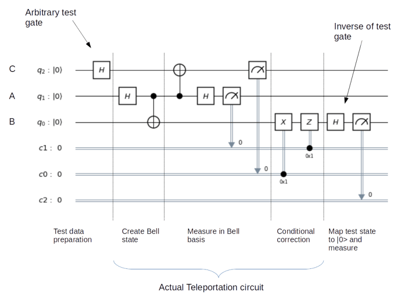
For our tests, we will use the description of Shor’s algorithm in terms of the quantum phase estimation procedure. Thus we have a primary register that we initialize in the state $|1\rangle$ and to which we apply a sequence of controlled multiplications by powers of a, and a working register, in which we do a quantum Fourier transform in the second step. The primary register needs to hold M=15, so we need four qubits there. For the working register, we use three qubits, which is the smallest possible choice, to keep the number of gates small.

The first step of our algorithm is controlled multiplication by a. However, this is greatly simplified by the fact that we apply this to exactly one state that we know upfront – the initial state $1 \rangle$ . Thus we only need to implement a unitary transformation which conditionally maps the state $|1 \rangle$ to the state $|a = 11 \rangle$ . In binary notation, eleven is 1011, and we therefore simply need to conditionally flip qubits 3 and 1. 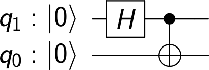We also need a Pauli X gate in the primary register to build the initial state $|1 \rangle$ from the fiducial state $|0\rangle$ and Hadamard gates in the working register to create the initial superposition. Thus the first part of our circuit looks as follows.

What about higher powers of a? This is easy – we know that a² is equal to one modulo M, and therefore the multiplication by a² modulo M is simply the identity transformation. The same is true for all even powers and so we are already done with the first part of our circuit – this is why we call the case a = 11 the easy case. The only thing that is left is to add the quantum Fourier transformation and a measurement to the working register. This gives us the following circuit (which can obviously be simplified, more on this later).

Now we can run this on a simulator. Before we do this, let us try to understand what we expect. We know that after measuring the working register, the value that we obtain is a multiple of 2³ / r = 8 / 2 = 4. Thus we expect to see peaks at 0 and four (binary 100). And this is actually what we get – the following histogram shows the output of an execution on the local QASM simulator integrated into Qiskit.

This is nice, our circuit seems to work correctly. So let us proceed and try this on real hardware. Before we do so, however, let us simplify our circuit a bit to reduce the number of gates needed and thus the noise level. First, we skip the final swap gates in the QFT circuit – this will change our expected output from 100 to 001, but we can keep track of this manually when setting up the measurement. Next, we have two Hadamard gates on w[2] that cancel and that we can therefore remove. And the Pauli X gate on p[0] is never really used and can be dropped. After these changes, we obtain the following circuit.

We can run this on the IBMQ hardware. As we require seven qubits in total, we need to do this on the 14 qubit model ibmq_16_melbourne. Here are the results of a test run, again as a histogram.

We see the expected peaks at 000 and 100, but also see some significant noise that is of course not present in the simulation. However, the probabilities to measure one of the theoretically expected values is still roughly twice as high as the probability of any of the other values.

The hard case – a = 7

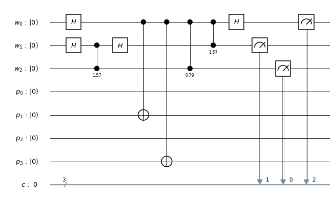
Having mastered the case a = 11, let us now turn to the case a = 7. The only change that we need to make is the circuit acting on the primary register. In the first part of the circuit, we can again make use of the fact that we only have to deal with one possible input, namely the initial state $|1 \rangle$ . The conditional multiplication by a maps this to $|7\rangle$ , and we can again implement this by two conditional bit flips, i.e. two CNOT gates.

The second part, the conditional multiplication by a² = 4 modulo M, requires a bit more gates. On a bit level, multiplication by four is a bit shift by two bits to the left. We can realize this as a sequence of two conditional swap gates, swapping the bits zero and two and the bits one and three. A conditional swap gate can be implemented by three CNOT gates, or, in QASM syntax,

gate cswap a,b,c
{
  cx c,b;
  ccx a,b,c;
  cx c,b;
}

We can also make a few simplifications by replacing CNOT gates with fixed values of the control qubit by either an inversion or the identity. We arrive at the following circuit.

This is already considerably more complex than for the case a = 11. When we add the QFT circuit and the measurements, we end up with the following circuit.

Now the period is four. Thus we expect peaks at all multiples of two, i.e. at all even values. And this is actually what we get when we run this on a simulator.

Now let us again see how we can optimize this circuit before trying it on real hardware. Again, there are a few additional simplifications that we can make to reduce the noise level. On w[2], we have a double Hadamard gate that we can remove. We can again dispose of the final swap gates and move the swap operation into the measurement. The last CNOT between p[1] and p[3] can be dropped as it does not affect the outcome. The same is true for the last CNOT between p[0] and p[2]. Thus we finally arrive at the following circuit.

And here is the result of running this on the 16 qubit IBM device.

Surprisingly, the noise level is not significantly worse than for the version with a = 11, even though we have a few more gates. We can clearly see that the probabilities to measure even values are significantly higher than the probabilities to measure odd values, corresponding to the period four.

So what did we learn from all this? First, our example was of course a toy model – we did code the circuit based on knowledge on the period and hard-coded the value of a. However, our example demonstrates the basic techniques to build circuits for the more general case. In real application, we could, given a number M, first determine a suitable value for a. The conditional multiplication by a is then acting as a permutation on the computational basis and can therefore be implemented by a sequence of (conditional) swap gates. The same is true for higher powers of a. So in theory, we have all the ingredients that we need to implement more general versions of the algorithm.

In practice, however, we will quickly reach a point where the number of gates exceeds the limit that we can reasonable implement given the current level of noise. So real applications of the algorithm in number ranges that are not tractable for classical digital computers will require advanced error correction mechanisms and significantly reduced noise levels. Still, it is nice (and fun) to see a toy version of the famous algorithm in action on a real device.

If you want to run the examples yourself, you can use my notebooks for the case a=11 and a=7.

References

1. L. Vandersypen, M. Steffen, G. Breyta, C. Yannoni, M. Sherwood, I. Chuang, Experimental realization of Shor’s quantum factoring algorithm using nuclear magnetic resonance, Nature Vol. 414, (December 2001)
2. P. Shor, Polynomial-Time Algorithms for Prime Factorization and Discrete Logarithms on a Quantum Computer, SIAM J.Sci.Statist.Comput. Vol. 26 Issue 5 (1997), pp 1484–1509, available as arXiv:quant-ph/9508027v2
3. R. Cleve, A. Ekert, C. Macchiavello, M. Mosca, Quantum Algorithms revisited, arXiv:9708016
4. A. Kitaev, Quantum measurements and the Abelian Stabilizer Problem, arXiv:quant-ph/9511026
5. J. Smolin, G. Smith, A. Vargo, Pretending to factor large numbers on a quantum computer, arXiv:1301.7007 [quant-ph]

Implementing the quantum Fourier transform with Qiskit

The quantum Fourier transform is a key building block of many quantum algorithms, from Shor’s factoring algorithm over matrix inversion to quantum phase estimation and simulations. Time to see how this can be implemented with Qiskit.

Recall that the quantum Fourier transform (or, depending on conventions, its inverse) is given by

$|x \rangle \mapsto \frac{1}{\sqrt{2^n}} \sum_s \eta^{xs} |s \rangle$

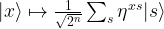
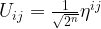
where $\eta$ is an 2ⁿ-th root of unity with n being the number of qubits in the register, i.e.

$\eta = \exp \frac{2\pi i}{2^n}$

How can we effectively create this state with a quantum circuit? They key to this is the observation (see the references below) that the result of the quantum Fourier transform can be written as a product state, namely as

$\sum_s \eta^{xs} |s \rangle = (|0\rangle + \eta^{2^{n-1} x}|1\rangle)(|0 \rangle + \eta^{2^{n-2}x}|1 \rangle) \cdots (|0 \rangle + \eta^x|1 \rangle)$

which you can easily verify by multiplying out the product and collecting terms.

Here we use the tensor product order that is prescribed by OpenQASM, i.e. the most significant bit is q[n-1]. This bit is therefore given by

$|0 \rangle + \eta^{2^{n-1}x} |1 \rangle$

Let us analyse this expression further. For that purpose, we decompose x into its representation as a binary number, i.e. we write

$x = \sum_{i=0}^{n-1} 2^i x_i$

with x_i being the binary digits of x. If we now multiply this by 2^n-1, we will get $2^{n-1} x_0$ plus a multiple of 2ⁿ. As $\eta$ is a root of unity, this multiple cancels out and we obtain that

$\eta^{2^{n-1}x} = \eta^{2^{n-1}x_0} = e^{\pi i x_0} = (-1)^{x_0}$

Thus, we can write the most significant qubit of the Fourier transform as

$|0 \rangle + (-1)^{x_0} |1 \rangle$

which is nothing but

$H |x_0\rangle$

Thus we obtain the most significant qubit of the quantum Fourier transform by simply applying a Hadamard gate to the least significant qubit of the input.

This is nice and simple, but what about the next qubit, i.e. qubit n-2? From the decomposition above, we can see that this is simply

$|0 \rangle + \eta^{2^{n-2}x} |1 \rangle$

Using exactly the same arguments as for the most significant qubit, we easily find that this is

$|0 \rangle + \eta^{2^{n-2}x_0} H |x_1 \rangle$

Thus we obtain this qubit from qubit 1 by first applying a Hadamard gate and then a conditional phase gate, i.e. a conditional rotation around the z-axis, conditioned on the value of x₀. In general, qubit n-j is

$|0 \rangle + \prod_{i < j - 1} \eta^{2^{n-j+i}x_i} H |x_{j-1}\rangle$

which is a Hadamard gate followed by a sequence of conditional rotations around the z-axis, conditioned on the qubits with lower significance.

So we find that each qubit of the Fourier transform is obtained by applying a Hadamard followed by a sequence of conditional rotations. However, the order of the qubits in the output is reversed, i.e. qubit n-j is obtained by letting gates act on qubit j. Therefore, at the end of the circuit, we need to revert the order of the qubits.

In OpenQASM and Qiskit, a conditional rotation around the z-axis is called CU1, and there are swap gates that we can use to implement the final reversing of the qubits. Thus, we can use the following code to build a quantum Fourier transformation circuit acting on n qubits.

def nBitQFT(q,c,n):
    circuit = QuantumCircuit(q,c)
    #
    # We start with the most significant bit
    #
    for k in range(n):
        j = n - k
        # Add the Hadamard to qubit j-1
        circuit.h(q[j-1])
        #
        # there is one conditional rotation for
        # each qubit with lower significance
        for i in reversed(range(j-1)):
            circuit.cu1(2*np.pi/2**(j-i),q[i], q[j-1])
    #
    # Finally we need to swap qubits
    #
    for i in range(n//2):
        circuit.swap(q[i], q[n-i-1])
    return circuit

Here is the circuit that this code produces for n=4. We can clearly see the structure – on each qubit, we first act with a Hadamard gate, followed by a sequence of conditional rotations with decreasing angle, conditioned on the less significant qubits, and finally reorder the qubits.

This is already a fairly complex circuit, and we need to find a way to test it. Let us look at the options we have. First, a quantum circuit is a unitary transformation and can be described by a matrix. In our case, it is especially easy to figure out what this matrix should be. Looking at the formula for the quantum Fourier transform, we find that the matrix describing this transformation with respect to the computational basis has the elements

$U_{ij} = \frac{1}{\sqrt{2^n}} \eta^{ij}$

The Qiskit frameworks comes with a simulator called the unitary_simulator that accepts a quantum circuit as input and returns the matrix describing that circuit. Thus, one possible test approach could be to build the circuit, run the unitary simulator on it, and to compare the resulting unitary matrix with the expected result given by the formula above. In Python, the expected result is produced by the following code

def qftMatrix(n):
    qft = np.zeros([2**n,2**n], dtype=complex)
    for i in range(2**n):
        for j in range(2**n):
            qft[i,j] = np.exp(i*j*2*1j*np.pi/(2**n))
    return 1/np.sqrt(2**n)*qft

and the test can be done using the following function

def testCircuit(n):
    q = QuantumRegister(n,"x")
    c = ClassicalRegister(n,"c")
    circuit = nBitQFT(q,c,n)

    backend = Aer.get_backend('unitary_simulator')
    job = execute(circuit, backend)
    actual = job.result().get_unitary()
    expected = qftMatrix(n)
    delta = actual - expected
    print("Deviation: ", round(np.linalg.norm(delta),10))
    return circuit

The outcome is reassuring – we find that the matrices are the same within the usual floating point rounding differences.

After passing this test, a next reasonable validation step could be to run the algorithm on a specific input. We know that the QFT will map the state $|0 \rangle$ into an equal superposition of all elements of the computational basis. Conversely, we therefore expect that if we start with such a superposition, the QFT will map the superposition onto $|0\rangle$ , at least up to a phase.

Let us try this out. Our test circuit will consist of a layer of Hadamard gates to create the equal superposition, followed by the QFT circuit, followed by a measurement. The resulting circuit for n=4 is displayed below.

It we run this circuit on the QASM simulator embedded into Qiskit, the result is as expected – for 1024 shots, we get 1024 times the output ‘0000’. So our circuit works – at least theoretically. But what about real hardware?

Let us compile and run the circuit targeting the IBM Q Experience 14 qubit device. If we dump the QASM code after compilation, we see that the overall circuit will have roughly 140 gates. This is already significant, and we expect to see some noise. To see how bad it is, I have conducted several test runs and plotted the results as a histogramm (if you want to play with this yourself, you will find the notebook on Github). Here is the output of a run with n=4.

We still see a clear peak at the expected result, but also see that the noise level is close to making the result unusable – if we did not know the result upfront, we would probably not dare to postulate anything from this output. With only three qubits, the situation becomes slightly better but is still far from being satisfactory.

Of course we could now start to optimize the circuit – remove cancelling Hadamard gates, remove the final swap gates, reorder qubits to take the coupling map into account and so on – but it becomes clear that with the current noise level, we are quickly reaching a point where even comparatively simple circuit will inflict a level of noise that is at best difficult to handle. Hopefully, this is what you expected after reading my posts on quantum error correction, but I found it instructive to see noise in action in this example.

References

1. M. Nielsen, I. Chuang, Quantum Computation and Quantum Information, Cambridge University Press 2010
2. R. Cleve, A. Ekert, C. Macchiavello, M. Mosca, Quantum Algorithms revisited, arXiv:9708016

Computational basis vector	Bell basis vector
$\|00 \rangle$	$\|\beta_{00} \rangle = \frac{1}{\sqrt{2}} (\|00 \rangle + \|11 \rangle)$
$\|01 \rangle$	$\|\beta_{01} \rangle = \frac{1}{\sqrt{2}} (\|01 \rangle + \|10 \rangle)$
$\|10 \rangle$	$\|\beta_{10} \rangle = \frac{1}{\sqrt{2}} (\|00 \rangle - \|11 \rangle)$
$\|11 \rangle$	$\|\beta_{11} \rangle = \frac{1}{\sqrt{2}} (\|01 \rangle - \|10 \rangle)$