Quantum phase estimation – the quantum algorithm Swiss army knife

When you are faced with a problem in linear algebra and have absolutely no idea what to do, an eigenvalue decomposition is the one thing that you would typically try first. In the world of quantum algorithms, the situation is similar – finding the eigenvalues of a matrix is a central building block of many quantum algorithm. The most important approach to finding the eigenvalues is called the quantum phase estimation algorithm.

The quantum phase estimation algorithm

In its most basic form, the quantum phase algorithm is used to find an eigenvalue of a unitary matrix assuming that we know an eigenvector (we will see later that this is in fact not necessarily needed for useful applications). So let us assume that we are given a unitary matrix U, implemented as a quantum circuit, and a quantum state $|\psi \rangle$ which is an eigenvector of U. As U is unitary, all eigenvalues are on the complex unit circle, and therefore the eigenvalue equation is

$U |\psi \rangle = e^{2\pi i \varphi} |\psi \rangle$

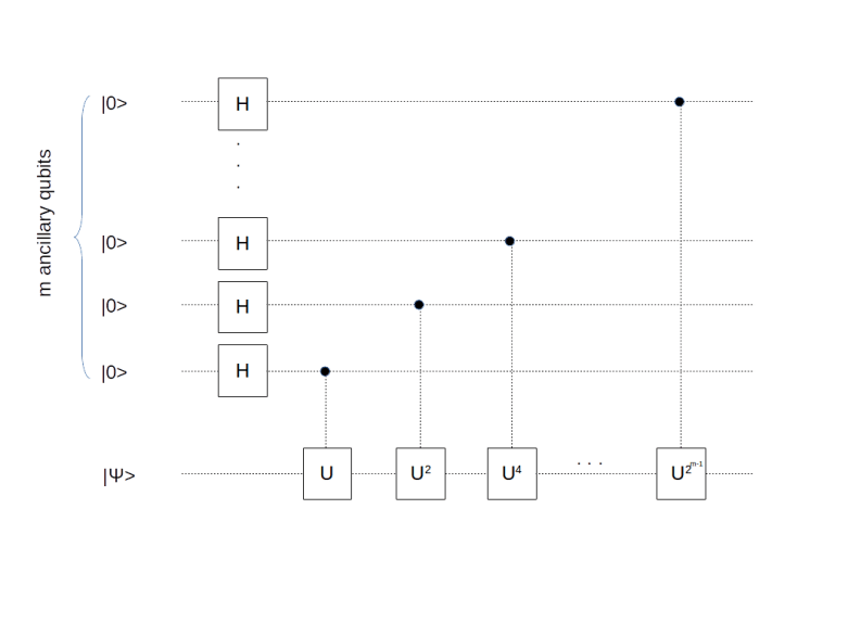
for some number $\varphi$ between zero and one. The quantum phase estimation is designed to determine (or at least approximate) the number $\varphi$ , i.e. the phase of the eigenvalue (hence the name).

The algorithm consists of two parts. Both parts operate on an ancillary working register and a register that we call the primary register. Let n denote the number of qubits in the primary register and m denote the number of qubits in the working register. We assume that the initial state in the primary register is the state $|\psi \rangle$ . The first step of the algorithm is to prepare the system in the state

$\frac{1}{\sqrt{2^m}} \sum_{k=0}^{2^m - 1} |k \rangle U^k |\psi \rangle$

How can we prepare this state? Given a state $|k \rangle$ , with binary digits k_i, we can of course write U^k as

$U^k = \prod_i \big[ U^{2^i} \big]^{k_i}$

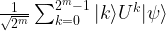
In other words, U^k is a sequence of conditional gates U^2ⁱ, conditioned on the i-th bit of k. Together with the usual approach to prepare an equal superposition of all $|k \rangle$ by using Hadamard gates, this argument shows that the desired state can be prepared by the following quantum circuit.

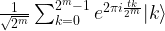
So far we have not yet used that the initial state $|\psi \rangle$ is an eigenstate. Let us do this now. We know that a power of U will act on $|\psi \rangle$ as multiplication by the corresponding power of the eigenvalue, hence

$\frac{1}{\sqrt{2^m}} \sum_{k=0}^{2^m - 1} |k \rangle U^k |\psi \rangle = \frac{1}{\sqrt{2^m}} \big[\sum_{k=0}^{2^m - 1} e^{2\pi i \varphi k} |k \rangle \big] \otimes |\psi \rangle$

This is interesting – our state turns out to be a product state (as the multiplication by a scalar can be pulled through the tensor product). To understand the first part of the product (i.e. the resulting state in the working register) in more detail, let us assume for a moment that the phase $\varphi$ is an exact multiple of 2^-m, i.e. that

$\varphi = \frac{t}{2^m}$

for some integer t. Then the state in the working register is

$\frac{1}{\sqrt{2^m}} \sum_{k=0}^{2^m - 1} e^{2\pi i \frac{tk}{2^m}} |k \rangle$

But this is simply the inverse quantum Fourier transform applied to the state $|t \rangle$ ! So we can obtain t and therefore $\varphi$ by applying a quantum Fourier transform to the state in the working register and doing a measurement. This is the quantum phase estimation algorithm.

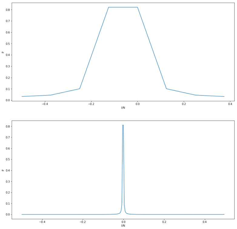
In most cases, the phase will of course not be an exact multiple of t / 2^m. However, with a bit more work (see for instance arXiv:quant-ph/9708016 or my own notes) one can see that the our result is still approximately true, i.e. if we run this algorithm, measure the value in the working register and divide by 2^m, we get a good approximation to the actual phase $\varphi$ . The precision of the estimation depends on the number of qubits m that we have in our working register. The following diagram demonstrates this for a specific example for two different values of m.

The x-axis shows the absolute deviation from the true value, the y-axis shows the probability for this deviation. The upper image corresponds to m=3. We see that there is a peak around zero, but still a substantial probability to have a significant error. The lower diagram shows the outcome for m=8. Here we see that the peak is very sharp, and so we obtain a very good approximation with high probability.

Shor’s algorithm as an instance of quantum phase estimation

Most of the time, the quantum phase estimation algorithm is used as a subroutine in a more general algorithm. A prominent example is Shor’s algorithm which – as we will now see – can be expressed as an application of the quantum phase estimation.

Recall that the quantum part of Shor’s algorithm is concerned with finding the period of a number a modulo M, where M is some large integer that we want to factor. Here we assume that a is a unit modulo M so that one of its powers is one. As a is a unit, the mapping

$U \colon |x \rangle \mapsto |ax \mod M\rangle$

is a unitary transformation U for x < M (which we can extend by the identity to a unitary transformation of the full Hilbert space). If r denotes the period of U, then clearly the fact that a^r = 1 modulo M implies that U^r = 1. Thus all eigenvalues of U are r-th roots of unity. In other words, if an eigenvalue has phase $\varphi$ , then $\varphi r$ is an integer. We can therefore use the phase estimation algorithm to obtain the period r.

There is one twist, however. To be able to apply the phase estimation algorithm, we need an eigenvector as an initial state, and it is far from clear how to prepare this. Fortunately, a deeper analysis (again see arXiv:quant-ph/9708016 or my own notes for all the details of this) shows that the state $|1 \rangle$ is a sum of eigenstates. Running the algorithm on this state will – by linearity – produce a state which is a superposition of states corresponds to different multiples of 2^m / r, and performing the measurement will choose one of these multiples. As in Shor’s original version of the algorithm, we can then use a continued fraction expansion to obtain the unknown period r. Thus, the following algorithm can be used to determine the period r.

Prepare a primary register in the state $|1 \rangle$
Apply the circuit shown above
Apply a quantum Fourier transform to the working register
Perform a measurement of the working register and call the result s – this will be close to a multiple of 2^m / r
Perform a continued fraction expansion to find the period r as in Shor’s original version of the algorithm

At the first glance, it looks as if we had found an alternative period finding algorithm, but if you actually draw up the circuit that realizes this algorithm, you will find – again see the references cited before – that this is not true, in fact the resulting circuit will be almost identical to the circuit for Shor’s version of the algorithm. Thus we have not found a new algorithm, but have found a different description of the same algorithm – period finding can be described as an instance of the phase estimation algorithm.

More applications

Of course factoring integers is not the only possible application of the quantum phase estimation. An obvious application is finding eigenvalues of Hamiltonians, i.e. energy eigenvalues – and in particular ground state energies – of physical systems. We have already touched on this possible application in a previous post on the quantum variational eigensolver.

Another application is based on the observation that if we start the algorithm with a superposition of eigenvectors, the measurement at the end of the algorithm will not only select an eigenvalue, but also an eigenvector. Thus we can use the algorithm to decompose a state into a superposition of eigenvectors. This can be used to solve linear equations of the form Ax = b for a given matrix A. In fact, if we can diagonalize A, then solving this equation becomes equivalent to division. Implementing this as a quantum algorithm is not as simple and straightforward as this description might suggest, as the division is a non-unitary operation, but it turns out that it can be approximated by a unitary transformation. The resulting algorithm is called the HHL-algorithm after its inventors Harrow, Hassidim and Lloyd, and has been published in this paper on the arxiv.

The HHL algorithm does not guarantee a quantum advantage for every matrix A, as it relies on a way to efficiently calculate the corresponding time evolution operators e^iAt. However, if for instance A is sparse and has low condition number (ratio between eigenvalues), the algorithm provides an exponential speedup over the best classical algorithms. An important application is deep machine learning, where efficient matrix inversion plays an important role – see for instance this paper by Zhao, Pozas-Kerstjens, Rebentrost, and Witte, as well as the corresponding source code. The details of the HHL algorithm are far from being trivial, and we will leave a more in-depth discussion to a future post.

Quantum phase estimation – the quantum algorithm Swiss army knife

The quantum phase estimation algorithm

Shor’s algorithm as an instance of quantum phase estimation

More applications

Published by christianb93

1 Comment

Leave a Comment Cancel reply

The quantum phase estimation algorithm

Shor’s algorithm as an instance of quantum phase estimation

More applications

Share this:

Like this:

Related

Published by christianb93

1 Comment

Leave a Comment Cancel reply