Mathematics – Page 3 – LeftAsExercise

Restricted Boltzmann machines

In the previous post, we have seen that a Boltzmann machine as studied so far suffers from two deficiencies. First, training is very slow as we have to run a Gibbs sampler until convergence for every iteration of the gradient descent algorithm. Second, we can only see the second moments of the data distribution and the learning rule ignores higher moments.

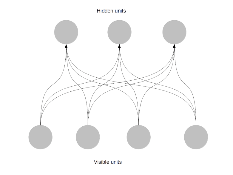
A class of networks called Restricted Boltzmann machines (RBM) has been designed to overcome these problems. An RBM is a Boltzmann machine with two additional architectural features. First, it has hidden units. This simply means that we split the set of all units in the network into two disjoint sets called visible units and the said hidden units. When we we train the network, we connect the data samples only to the visible units. The hidden units, however, also follow the dynamical rules of the network and serve as latent variables – you can think of them as additional parameters of the network which are adapted during training but are not directly prescribed by the training set, similar to a hidden layer in a feed-forward neuronal network.

Second, in a restricted Boltzmann machine, certain restrictions on the weights are in effect. Specifically, we only allow hidden units to be connected to visible units and vice versa, so there are no connections between hidden units and no connections between visible units. Effectively, a restricted Boltzmann machine is therefore organised in two layers – one layer containing the hidden units and one layer containing the visible units, as shown below.

What does this imply for the mathematical description of the network? In fact, we will see that this simplifies things considerably. First, corresponding to the differentiation between hidden and visible units, our index set can be written as

$\{ 1, \dots, N \} = I_v \cup I_h$

so that unit i is a hidden unit if i is in the set $I_v$ and a hidden unit if i is in the set $I_h$ . Second, it is common to use 0 and 1 as states instead of -1 and +1. Our state space then splits

$\{ 0, 1\}^N = {\mathcal S} = {\mathcal V} \times \mathcal {H}$

and correspondingly we can write any state as

$s = (v,h)$

where v specifies the state of the visible units and h the state of the hidden units. As only visible units correspond to actual input, the purpose of the training phase is now to adjust the marginal distribution

$P(v) = \sum_h P(v,h) = \frac{1}{Z} \sum_h e^{-\beta E(v,h)}$

such that is it as close as possible to the empirical distribution of the test data.

The expression for the energy also simplifies greatly, as all terms involving only hidden units and only visible units disappear. If we replace the matrix W that contains all connections by a reduced matrix – that we again call W – that only contains the remaining connections between visible and hidden units, we can express the energy as

$E(v,h) = - \sum_{i \in I_v, j \in I_h} W_{ij} v_i h_j$

In addition, we will now also add an explicit bias to both the hidden and visible units, so that our full energy is

$E(v,h) = - \sum_{i \in I_v, j \in I_h} W_{ij} v_i h_j - \sum_i v_i b_i - \sum_j h_j c_j$

Of course the matrix W is now no longer symmetric and not even quadratic (as the number of hidden units will in general not be the same as the number of visible units).

We can now again calculate the update rules as before. First, we write down the likelihood function

$l({\mathcal D} | W) = - \frac{1}{K} \ln P({\mathcal D} | W) = - \frac{1}{K} \sum_k \ln \sum_h e^{-\beta E(v^{(k)},h)}+ \ln Z$

where now $v^{(k)}$ is the k-the sample point corresponding to a set of values for the visible units.

Again we will need the derivatives of this with respect to the weights. For the second term – the logarithm of the partition function – we have already seen in the last post how this works. Recalling the results from this post, we easily find that

$\frac{\partial}{\partial W_{ij}} \ln Z = - \beta \langle \frac{\partial E}{\partial W_{ij}} \rangle_P = \beta \langle v_i h_j \rangle_P$

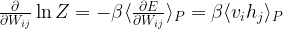
so that the derivative is again an expectation value which we could try to approximate using a sample of the model distribution. The first term requires a bit more work. Let us first calculate

$\frac{\partial }{\partial W_{ij}} \ln \sum_h e^{-\beta E(v,h)} = \frac{1}{Z P(v)} \sum_h \frac{\partial }{\partial W_{ij}} e^{-\beta E(v.h)}= - \beta \sum_h \frac{\partial E(v,h)}{\partial W_{ij}} P(h | v)$

But this is again an expectation value, this time it is an expectation value with respect to the conditional distribution of the hidden units given the visible units.

$\frac{\partial }{\partial W_{ij}} \ln \sum_h e^{-\beta E(v,h)} = - \beta \langle \frac{\partial E(v,h)}{\partial W_{ij}} \rangle_{P(\cdot | v)}$

The derivative of the energy with respect to the weights is as above, and we finally obtain the following update rule for the weights:

$\Delta W_{ij} = \lambda \beta \left[ \langle \langle v_i h_j \rangle_{P(\cdot | v)} \rangle_{\mathcal D} - \langle v_i h_j \rangle_P \right]$

Note that the first term is a double expectation value – for each sample $v^{(k)}$ for the visible units, we use the expectation value under the conditional distribution over the hidden units given this value for the visible units.

Now let us start to simplify this expression a bit further, leveraging the restrictions on the geometry of the network. Let us first try to find an expression for the conditional probability

$P(h_j = 1 | v)$

This is in fact easy to calculate in our situation. As the state of a hidden unit does not depend on the other hidden units, but only on the visible units, we find that

$P(h_j = 1 | v)= \sigma(\beta (\sum_i W_{ij} v_i + c_j)) = \sigma(\beta a_j)$

where

$a_j = \sum_i W_{ij} v_i + c_j$

is the activation of the hidden unit j. Using this, we can already simplify the first term in the update rule as follows:

$\langle v_i h_j \rangle_{P(\cdot | v)} = \sum_h P(h | v) v_i h_j = v_i \sum_{h : h_j = 1} P(h | v)$

But this is of course nothing but

$v_i P(h_j = 1 | v)$

so that we eventually find

$\langle v_i h_j \rangle_{P(\cdot | v)} = v_i \sigma (\beta a_j)$

A similar argument works for the second term in the update rule. We have

$\langle v_i h_j \rangle_P = \sum_v \sum_h v_i h_j P(v,h) = \sum_v v_i P(v) \sum_h h_j P(h | v)$

Now the second term sum is again the conditional probability for $h_j$ to be one given v, so that this turns into

$\langle v_i h_j \rangle_P = \sum_v v_i P(v) \sigma(\beta a_j) = \langle v_i \sigma(\beta a_j) \rangle_{P(v)}$

We therefore finally obtain the following simplified update rule.

$\Delta W_{ij} = \beta \left[ \langle v_i \sigma(\beta a_j) \rangle_{\mathcal D} - \langle v_i \sigma(\beta a_j) \rangle_{P(v)} \right]$

Thus again, we see that the gradient is composed of two terms, which we call the positive phase and the negative phase. In each phase, we sample the same expression, once over the data distribution and once over the marginal distribution.

How do we actually calculate these terms? The positive phase is easy – we have written this as an expectation value, but it is nothing but an ordinary sum. For each vector in the sample, we calculate the activation of the hidden unit j, apply the multiplication by $\beta$ and the sigmoid function and multiply the result with the value of the visible unit. So this is in fact an easily calculated analytical expression.

Whereas we have found an analytic expression for the positive phase, there is no obvious analytic expression for the negative phase, so we again need a sampling procedure to calculate this term. At this point, the special structure of the network again helps to make the sampling easier. Suppose we wanted to apply an ordinary Gibbs sampler, where instead of choosing the neuron that we update next randomly, we cycle sequentially through all the neurons. We could then do all the hidden neurons first and then continue with the visible units. Now, as the visible units only depend on the hidden units and vice versa, we could as well update all hidden units in parallel and then all visible units in parallel, using that as in the case of hidden units, the conditional probability for a visible unit to be one can be expressed as

$P(v_i = 1 | h) = \sigma(\beta (\sum_j W_{ij} h_j + b_i))$

This procedure is called Gibbs sampling with block updates. It is also obvious that sampling from the joint distribution $P(v,h)$ in this way and then ignoring the values of the hidden units in this way gives a sampler for the marginal distribution.

Therefore our algorithm to calculate the second term of the update rule would be as follows. We would start with some value for the visible units. Then we would calculate the probability that each hidden unit is on given these values for the visible units and update the hidden units according to this distribution. We would then use the new values for the hidden units, calculate the conditional distribution of the visible units and update the visible units according to this distribution. This would constitute a full Gibbs sampling step. We would repeat this process until convergence is reached and then sample for a few steps to calculate the expectation values above. Plugging this into the update rule and calculating the first term analytically, we would then obtain the needed update for the weights.

So it looks like we are back to our old problem – to calculate one weight update during the gradient descent procedure, we have to run a Gibbs sampler to convergence. Fortunately, it turns out that several approximations exist that make this calculation feasible. Next, we will look at two of these approaches – constrastive divergence and its companion persistent contrastive divergence (PCD). We will then implement both algorithms in Python and try it out, first on a small sample set and then finally on the MNIST data set. But this post has already grown a bit lengthy – so let us save this for the next post in this series.

Turn on the heating – from Hopfield networks to Boltzmann machines

In my recent post on Hopfield networks, we have seen that these networks suffer from the problem of spurious minima and that the deterministic nature of the dynamics of the network makes it difficult to escape from a local minimum. A possible approach to avoid this issue is to randomize the update rule. Intuitively, we want to move into a direction of lower energy most of the time, but sometimes allow the network to move a different direction, so that there is a certain probability to move away from a local minimum.

In a certain sense, a Boltzmann machine is exactly this – a stochastic version of a Hopfield network. If we want to pursue the physical analogy further, think of a Hopfield network as an Ising model at a very low temperature, and of a Boltzmann machine as a “warm” version of the same system – the higher the temperature, the higher the tendency of the network to behave randomly and to escape local minima. As for the Hopfield network, there are different versions of this model. We can allow the units to take any real value, or we can restrict the values to two values. In this post, we will restrict ourselves to binary units. Thus we consider a set of N binary units, taking values -1 and +1, so that our state space is again

$S = \{ -1, +1 \}^N$

Similar to a Hopfield network, each unit can be connected to every other unit, so that again the weights are given by an N x N matrix W that we assume to be symmetric and zero along the diagonal. For a state s, we define the energy to be

$E(s) = - \frac{1}{2} \langle s, Ws \rangle$

This energy defines a Boltzmann distribution on the state space, given by

$P(s) = \frac{1}{Z} e^{-\beta E(s)}$

Now our aim is to adjust the weights such that this distribution is the best possible approximation to the real distribution behind the training data.

How do we measure the distance between the current distribution and the target distribution? A common approach to do this is called the maximum likelihood approach: given a set of weights W, we try to maximize the probability for the training data under the distribution given by W. For convenience, one does usually not maximize this function directly, but instead minimizes minus the logarithm of this probability, divided by the number K of samples. In our case, we therefore try to minimize the loss function

$l({\mathcal D} | W) = - \frac{1}{K} \ln P({\mathcal D} | W)$

Now let us assume that our sample is given by K data points that we denote by $s^{(k]}$ . Assuming that the sample states are independent, we can write the probability for the data given the weights W as the product.

$P({\mathcal D} | W) = \prod_k P(s^{(k)} | W)$

Using the definition of the Boltzmann distribution and the partition function Z, we can therefore express our loss function as

$l({\mathcal D} | W) = \ln Z + \frac{\beta}{K} \sum_k E(s^{(k)})$

where $s^{(k)}$ is the k-th sample point, where we assume that all sample points are drawn independently.

Now how do we minimize this function? An obvious approach would be to use the gradient descent algorithm or one of its variants. To be able to do this, we need the gradient of the loss function. Let us first calculate the partial derivative for the first term, the logarithm of the partition function. This is

$\frac{\partial}{\partial W_{ij}} \ln Z = \frac{1}{Z} \sum_s \frac{\partial}{\partial W_{ij}} e^{-\beta E(s)} = - \beta \frac{1}{Z} \sum_s e^{-\beta E(s)} \frac{\partial}{\partial W_{ij}} E(s) = - \beta \sum_s P(s) \frac{\partial}{\partial W_{ij}} E(s)$

Now the sum on the right hand side of this equation is of the form “probability of a state times a function of this state”. In other words, this is an expectation value. Using the standard notation for expectation values, we can therefore write

$\frac{\partial}{\partial W_{ij}} \ln Z = - \beta \langle \frac{\partial}{\partial W_{ij}} E(x) \rangle_P$

If you remember that expectation values can be approximated using Monte Carlo methods, this is encouraging, at least we would have an idea how to calculate this. Let us see whether the second term can be expressed as an expectation values as well. In fact, this is even easier.

$\frac{\partial}{\partial W_{ij}} \frac{\beta}{K} \sum_k E(s^{(k)}) = - \frac{\beta}{2} \frac{1}{K} \sum_k s_i^{(k)} s_j^{(k)}$

Now this is again an expectation value – it is not an expectation value under the model distribution (the Boltzmann distribution) but under the empirical distribution of the data set.

$\frac{\partial}{\partial W_{ij}} \frac{\beta}{K} \sum_k E(s^{(k)}) = - \frac{\beta}{2} \langle s_i s_j \rangle_{\mathcal D}$

Finally, our expression for the first term still contains the derivative of the energy, which is easily calculated. Putting all of this together, we now obtain a formula for the gradient of the loss function which is maybe the most important single formula for Boltzmann machines that you need to remember.

$\frac{\partial}{\partial W_{ij}} l({\mathcal D} | W) = - \frac{\beta}{2} \left[ \langle s_i s_j \rangle_{\mathcal D} - \langle s_i s_j \rangle_P \right]$

When using the standard gradient descent algorithm, this expression for the gradient leads to the following update rule for the weights, where $\lambda$ is the step size.

$\Delta W_{ij} = \frac{1}{2} \lambda \beta \left[ \langle s_i s_j \rangle_{\mathcal D} - \langle s_i s_j \rangle_P \right]$

Let us pause for a moment and reflect what this formula tells us. First, if we have reached our goal – model distribution and sample distribution are identical – the gradient is zero and the algorithm stops.

Second, the first term is essentially the Hebbian learning rule that we have used to train our Hopfield network. In fact, this is the weighted sum over the product $s_i s_j$ across all sample points, i.e. we strengthen a connection between two units if the two units are strongly correlated in the sample set, and weaken the connection otherwise. The second term is a correction to the Hebbian rule that does not appear in a Hopfield network.

The third point that we can observe is a bit more subtle. To explain it, assume for a moment that the data has been normalized (which is very often done in actual applications) so that its average is zero, in other words such that the expectation values

$\langle s_i \rangle_{\mathcal D}$

of the coordinates are all zero. For the Boltzmann distribution, this will be the case anyway as the distribution is symmetric in s (and it would therefore not even make sense to try to achieve convergence with unnormalized data). Thus the two terms that appear in the above equation are simply the elements of the covariance matrix under empirical and model distribution. This implies that a Boltzmann machine is not able to distinguish two distributions that have the same second moments as the covariance matrix is all that it sees.

That is a bit disappointing as it limits the power of our model significantly. But this is not the only problem with Boltzmann machines. Whereas we could easily calculate the first term in our formula for the weight change, the second term is more difficult. In our discussion of the Ising model, we have already seen that we could use Gibbs sampling for this, but would need to run a Gibbs sampling chain to convergence which can easily take one million steps or more for large networks. Now this is embedded into gradient descent which is by itself an iterative algorithm! Imagine that one single gradient descent step could take a few minutes and then remember that we might need several thousand of these steps and you see that we are in trouble.

Fortunately, help is on the way – with a slightly simplified model called restricted Boltzmann machines, both problems can be solved. I will look at this class of networks in my next post in this series. If you do not want to wait until then, you can take a look at my notes on Boltzmann machines that also give you some more background on what we have discussed in this post.

Before we close, let me briefly describe what we could do with a Boltzmann machine if we had found a way to train it. Similar to a Hopfield network, Boltzmann machines are generative models. Thus once they are trained, we can either use them to create samples or to correct errors. If, for instance, each unit corresponds to a pixel in an image of a handwritten digit, we could sample from the model to obtain artificially created images that resemble handwritten digits. We could also use the network for pattern completion – if we have an image where a few pixels have been erased, we could start the network in the state given by the remaining pixels and some random values for the unknown pixels and hope that it converges to the memorized state, thus reconstructing the unknown part of the picture. However, specifically for restricted Boltzmann machines, we will see that an even more important application is to be used as feature extractor in deep layered networks.

So there are good reasons to continue analyzing these networks – so join me again in my next post when we discuss restricted Boltzmann machines.

The Ising model and Gibbs sampling

In the last post in the series on AI and machine learning, I have described the Boltzmann distribution which is a statistical distribution for the states of a system at constant temperature. We will now look at one of the most important applications of this distribution to an actual model, the Ising model.

This model was proposed by W. Lenz and first analysed in detail by his student E. Ising in his dissertation (of which [1] is a summary) to explain ferromagnetic behavior. In Isings model, a solid, like a piece of iron, is composed of a large number N of individual particles, each of them at a fixed location. A particle acts as a magnetic dipole that can be oriented in two different ways, corresponding to the different orientations of its spin. Ignoring the spatial structure for the time being, we can thus describe the state of the model as a point in the state space

${\mathcal S} = \{ -1, 1\}^N$

We denote the elements of the state space by s and the i-th spin by $s_i \in \{-1,1\}$ where a value of +1 is interpreted as “spin up” and a value of -1 as “spin down”.

Now, in general, a magnetic dipole which is exposed to a magnetic field B and has a magnetic dipole moment m will have a potential energy

$E = - m \cdot B$

which is the scalar product of m and B, i.e. the state of minimum energy is the one where the dipole is oriented along the magnetic field. In a solid, there are two sources for the magnetic field that act on each particle – there might be an external magnetic field H and there might be an interaction with the other magnetic dipoles in the model. We therefore model the total energy of a state s as

$E(s) = - \frac{1}{2} \sum_{i,j} J_{ij} s_i s_j - \sum_j h_j s_j$

where $J_{ii} = 0$ (i.e. we exclude self-interactions).

Here the coefficient $h_j$ represents the external field acting on the particle at position j. The matrix J represents the interactions between the particles. In Isings original model, only nearby particles interact. In two dimensions, for instance, we think of the particles as being located on a grid and each particle has four neighbors: the particles immediately above and below it and the particles on the left and on the right. We can define a model which has a boundary or we can think of the grid as being toroidal, i.e. wrapping around.

We now consider the system as being in contact with a heat bath at a certain temperature T, i.e. the system can exchange internal energy with a thermal reservoir, leading to fluctuations in the orientations of the particles. This appears to be a reasonable model, we could, for instance, consider a comparatively small part of a solid and take the surrounding, much larger solid as the heat bath. The probability for the system to be in a state s is therefore given by the Boltzmann distribution:

$p(s) = \frac{1}{Z} e^{-\beta E(s)}$

The macroscopic quantities that are of primary interest are of course the average energy, but also the magnetization

$M(s) = \frac{1}{N} \sum_i s_i$

and its average value. At high temperatures and for H = 0, we expect that roughly half of the spins should be oriented in either direction, so the average magnetization should be zero. If we add an external field, then of course most of the dipoles will be aligned in the direction of this field, so the magnetization will be close to one or minus one. This fact – magnetization of a solid in the presence of an external magnetic field – is called paramagnetism. It turns out that for some materials, a non-zero magnetization can occur even if the external field is zero, as long as the temperature is below a certain value called the critical temperature – this behavior is known as ferromagnetism. Explaining this macroscopic behavior by a statistical model was the original intention of Isings work.

Now how do we actually evaluate our model? Our aim is to determine – for instance – the average magnetization at a given temperature. To do this naively, we would have to calculate the probabilities for all possible states s. Unfortunately, the number of states grows exponentially with the number N of particles. Suppose we wanted to use a toy model with only 40 x 40 spins – this is very small compared to the number of particles in an average macroscopic solid. As N = 1600 in this case, we would have $2^{1600}$ different states, which is roughly $10^{482}$ . Comparing this to the estimated age of the universe in seconds ( $4 \cdot 10^{17}$ , see for instance this page), it is obvious that this is not a good idea.

However, we can try to approximate the average magnetization by using a sufficiently large sample. Thus we try to find a set of states $s_i$ which is large, but doable – maybe a few million – and hope, based on the law of large numbers, that the sample average, i.e. the sum $\sum_i M(s_i)$ , will provide a good approximation for the real value. This approach is sometimes called Monte Carlo integration and the workhorse of computational statistical mechanics.

How, then, do you create that sample? The answer is easy to write down, but difficult to motivate without the necessary background on Markov chains. Thus I will simply state the algorithm which is called Gibbs sampling and leave the theoretical background to another post (for the mathematically inclined reader, it is worth mentioning that the sample produced by the Gibbs sampler is not independent, but the law of large number still holds).

Before we can phrase the algorithm, we need another preparational step – we need to calculate a conditional probability. Suppose that the system is in a state s and we have chosen an arbitrary coordinate i. We can then ignore the actual state of the spin $s_i$ and ask for the conditional probability that this spin points upwards given all other spins. A not too difficult calculation (which is carried out in detail for instance in my notes) shows that this conditional probability is given by

$P(s_i = 1 | \{ s_j\}_{j \neq i}) = \sigma(2 \beta ( \langle J_i, s \rangle + h_i))$

Here $J_i$ denotes the i-th row of the matrix J and the brackets denote the ordinary scalar product. With this expression, a single Gibbs sampling step now proceeds as follows, given a state s.

Randomly pick a coordinate i
Calculate the conditional probability $P = P(s_i = 1 | \{ s_j\}_{j \neq i})$ using the formula above
Draw a real number U between 0 and 1 from the uniform distribution
If U is at most equal to P, set the spin at position i to +1, otherwise set it to -1

The algorithm then starts with a randomly chosen state and subsequently applies a large number of Gibbs sampling steps. After some time, called the burn-in time, the states after each step then form the sample we are looking for.

After all that theory, let us now turn to the practical implementation. We will restrict ourselves to the original model, i.e. $J_{ij} = 1$ if particles i and j are neighbors and zero otherwise, and also set the magnetic field to zero. The Gibbs sampling algorithm as outlined above is straightforward to implement in Python. You can get my code from GitHub as follows.

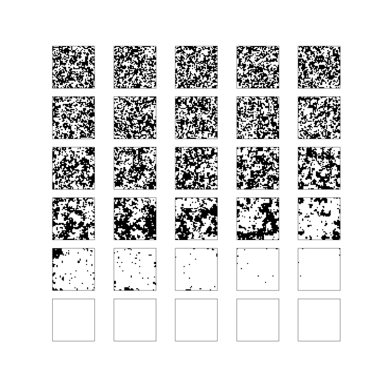
$ git clone https://github.com/christianb93/MachineLearning.git

In the newly created directory MachineLearning, you should then see a file Ising.py. Run this as follows.

$ python IsingModel.py

This will create a new temporary directory with a name that is unique and specifies the run (on Linux / Unix systems, you will find the newly created directory in /tmp/. In this subdirectory, you will find three files. A file with extension .txt summarizes the parameters of the run. The file that ends with IsingPartI.png displays the simulation results. An example is

Each of the little images represents one final state for a given temperature. In this example, a grid of 40 x 40 spins was calculated. The temperature was slowly decreased from 6.0 down to 0.2 in steps of 0.2. For each temperature, 4 million simulation steps were done, then the resulting grid was captured. The top row represents, from the left to the right, the temperatures 6.0, 5.8, 5.6, 5.4 and 5.2. Here we see the expected behaviour – patterns with roughly half of the particles in a spin-up position and half of the particles in a spin-down orientation.

In the bottom row of the diagram, that corresponds to the temperatures 1.0, 0.8, 0.6, 0.4 and 0.2, we also see the expected behavior for very low temperatures – all spins are oriented in the same direction. However, starting at temperatures 1.8, we see that large scale patterns start to emerge. especially for the temperatures 2.2 and 2.4 (rightmost pictures in the fourth row from the top). For these temperatures, entire connected regions display the same orientation of the spins and thus a non-zero mean magnetization. As the temperature rises, these patterns dissolve again.

This behaviour is typical for a so-called critical point and is what Ising was searching for. Ironically, Ising, who of course did not have the computational devices to run a simulation, concluded in his paper wrongly that this would not happen. Critical points are of great interest not only in statistical mechanics, but also in quantum field theory – we will not be able to explore this connection further, but it demonstrates how important the Ising model has become as a playground to bring together various branches from physics, computer science and mathematics.

The program has lots of parameters to play with – with the default values, for instance, it calculates comparatively small grids with 20 x 20 spins, so that a small number of iterations is sufficient, for larger grids you will need several million iterations. I recommend to play with this a bit to get a feeling for what happens. The image at the top of this article, for instance, was generated with the following command line:

$ python IsingModel.py --show=1 --N=160000 --rows=400 --cols=400 --steps=100000 --Tmax=2.4 --Tmin=1.7

and ran for roughly 13 minutes on my PC.

It is worth mentioning that neither the Gibbs sampling algorithm nor the chosen implementation are optimized. In fact, there are other algorithms like the exact sampling algorithm (see for instance [2]) that are providing much better results, and also the implementation could be improved greatly, for instance by using a Metropolis-Hastings checkerboard algorithm to allow for high parallelization and GPU computing (see for instance [3]). However, as understanding Gibbs sampling is vital for understanding Boltzmann machines, I have chosen to use a down-to-earth Gibbs sampling approach for this post – after all, its main purpose is not to gain new physical insights from simulation results but to get acquainted with Gibbs sampling as a standard sampling method, and, as always, to have some fun.

If you would like to learn more on the Ising model, please have a look at my notes that provide more details, show how to compute the conditional probability used for the Gibbs sampling and also cover the one-dimensional Ising model.

In the meantime, you might want to take a look at the beautiful article of J. Harder on WordPress who has some more sample pictures and a very interesting application of convolutional neuronal networks that he trained to be able to determine the temperatue at which the simulation was run from the visual representation of the simulation result.

References

1. E. Ising, Beitrag zur Theorie des Ferromagnetismus,
Zeitschrift f. Physik, Vol. 31, No.1 (1924), 253-258
2. D. MacKay, Information Theory, Inference and Learning Algorithms, Cambridge University Press, Cambridge 2003
3. M. Weigel, Simulating spin models on GPU, Computer Physics Communication 182 (2011), 1833-1836

Boltzmann machines, spin, Markov chains and all that

The image above displays a set of handwritten digits on the left. They look a bit like being sketched on paper by someone in a hurry and then scanned and digitalized, not very accurate but still mostly readable – but they are artificial, produced by a neuronal network, more precisely a so called restricted Boltzmann machine.

On the right hand side, you see the (core part of) the code that has been used to produce this image. These are about forty lines of code, and there is some code around it which is not shown, but stripping off all the comments and boilerplate code, we could probably fit the algorithm into less than fifty lines of code.

I found this contrast always fascinating. Creating something that resembles handwritten digits sounds incredibly complex, but can be done with an algorithm that can be quenched into a comparatively short program – how does that work? So I started to dig deeper, trying to understand neuronal networks in general and in particular Boltzmann machines – the mathematical foundations, the algorithm and the implementation.

Boltzmann machines are a rather special class of neuronal networks that have a reputation of being hard to train, but are important from a theoretical point of view, being closely related to seemingly remote fields like thermodynamics, statistical mechanics and stochastical processes. That makes them interesting, but also hard to understand. I embarked on that journey a couple of months ago, and I thought it would be nice to create a series of blog posts on this. My current thinking is to have one or two posts on each of the following topics over the next couple of weeks.

Overview – what are Boltzmann machines (this post)
Background from statistical mechanics and the Boltzmann distribution
The Ising model and Gibbs sampling
Hopfield networks: theory
Hopfield networks: practice
From Hopfield networks to Boltzmann machines
Restricted Boltzmann machines
Contrastive divergence and PCD
Implementation with TensorFlow
Basics of Markov chains
Finite Markov chains and recurrent Markov chains
The Metropolis Hasting algorithm

This is a lot of content, and please do not expect to see one post every other day. But maybe I should just start and we will see how it goes….

So let me try to roughly sketch what a Boltzmann machine is. First, it is a neuronal network. As such it is composed of units that can be compared to the neurons in the nervous system. Similar to a neuron, each unit has an input and an output. The output of a neuron can serve as input for another neuron. In general, every neuron receives inputs from many other neurons and delivers outputs to many other neurons.

The diagram above shows a very simple neuronal network. It consists of four neurons. The three of them on the left serve as input to the network. Think of them as the equivalent of cells in – say – your visual cortex that are activated by some external stimulus. The cell on the right is the output of the network. Its activation is computed based on the outputs of the neurons on the left and some parameters of the network called the weights which model the strength of the connection between the neurons and which we denote by $w_i, i = 0, 1, 2$ , as follows.

$o = \sigma(w_0 x_0 + w_1 x_1 + w_2 x_2) = \sigma(w^T X)$

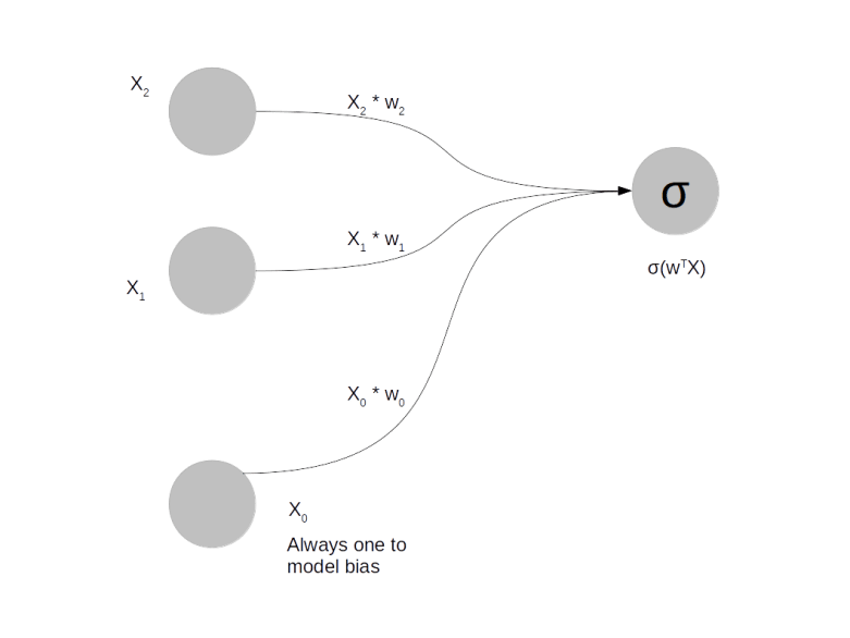
Here $\sigma$ is a function called the activation function and $X$ is the vector that is formed by $x_0, x_1$ and $x_2$ . There are a few standard choices for the activation function, a common one being the sigmoid function.

How is such a network applied? Let us look at this for a problem which is the “Hello World” of machine learning – recognition of handwritten digits. In that problem, you start with a collection of digitized images of handwritten digits, like those that are known as the MNIST database. These images have 28×28 = 784 pixels. We want to design a neuronal network that can classify these images. Such a network should consequently have 784 input units and 10 output units (bear with me that I did not produce a picture of that network, even though it would probably be fun to do this with Neo4J). We present an image to the network by setting the value of the input unit i to the intensity of pixel i. Our aim is to adjust the weights in such a way that if the image represents digit n, only output n is significantly different from zero. This will allow us to classify unknown images – we simply present the image to the network and then see which output is activated.

But how do we find the correct values for the weights? We need weights that connect each of the ten output units to each of the 784 input units, i.e. we have 7840 weights. Thus we are looking for a point in a 7840 dimensional vector space – not easy. Here the process of training comes into play. We take our set of sample images and present them to the network, with initially randomly chosen weights. The output will then not be what we want, but differ from the target output by an error. That error can be expressed as a function of the weights. The task is then to find a minimum of the error function, and there are ways to do this, most notably the procedure which is known as gradient descent.

As the name suggests, we need the gradient of the error function for that purpose. Fortunately, for the type of neuronal network that we have sketched so far, the gradient can be computed fairly easily – in fact the activation function is chosen on purpose to make dealing with the derivatives easy. We end up with a comparatively simple training algorithm for this type of network and maybe I will show how a simple implementation in Python in a later post – but for now let us move on to Boltzmann machines.

Boltzmann machines or more precisely restricted Boltzmann machines (RBMs) are also composed of units and weights, but work a bit differently. There are inputs, which are usually called visible units. But there are no classical outputs. Instead, there is a layer of units that is connected to the visible units and is called hidden units, as shown in the following picture.

In the example of handwritten digits again, you would again have 784 visible units. However, the hidden units would not obviously correlate with the digit represented by the input. Instead, you would have a more or less arbitrary number of hidden units, say 300.

During training, you present the network one image, again by setting the values of the visible units (the input) to the pixel intensities. You then compute the value of the hidden units – but you do not do this deterministically, but bring in some random element. Roughly speaking, if the combined input to a hidden unit is p, you set the value of the unit to one with probability p. Then this process is repeated, this time starting from the hidden units. This gives you certain values for the visible units. You then compare this value to the original value and try to adjust the weights such that you get as closely as possible to the original input (this is not exactly true and a not very precise description of one of the possible learning algorithms called contrastive divergence, but we will get more precise later on).

If you succeed, you will be able to reconstruct the value of the visible units from the values of the hidden units. But there are less hidden units, so that the network has apparently learned a condensed representation of the input that still captures the essence of the input. In the case of digits, you can visualize the state of the network after training and obtain something like

These are visualizations of the weights connected to some of the hidden units of a Bolzmann machine after the training phase. We can see that some of the units have appearantly “learned” some characteristic features of the digits, like the vertical stroke that appears in the digits one and seven. These features can be used for several purposes.

First, we can use the features as input for other neuronal networks. We now have only 300 inputs instead of originally 784, and that might simplify the problem a bit and make the process of training the next network easier.

Or, we could start with some random values for the hidden units and calculate the resulting values of the visible units to create sample images – and in fact this is basically what I have done to produce the samples at the top of this post (using an algorithm called PCD, but we will get to this).

Note that Boltzmann machines differ significantly from the type of neural network that we have considered earlier. One major difference is that to train a Boltzmann machine, you do not need to know the digit that the image represents. At no point have we used the information that the images in our database represent ten different digits – that information was not used in the design of the network nor during the training. This approach to machine learning is called unsupervised learning and is obviously very versatile – you do not have to tell the machine what the structure of the data is, it will detect the features independently.

Second, a Boltzmann machine can not only classify images, but can also create images that resemble a given set of input data. That can be used to reconstruct partially available images or to create new images from scratch – networks with this ability are called generative networks.

The price we have to pay for this is that Boltzmann machines are hard to train. The point is that we can still define some sort of error function, but we cannot easily calculate its gradient – there is no straightforward analytic expression for it that could be evaluated within a reasonable amount of time (if you know statistical physics a bit, that might remind you of the partition function, and that is more than pure coincidence, as I will show you in a later post). So we need to approximate the gradient. Technically, the gradient is an integral

$\int f(x) dx$

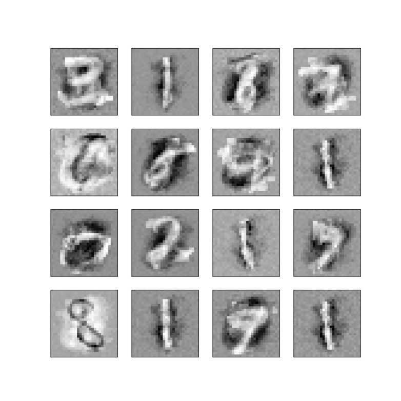
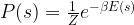
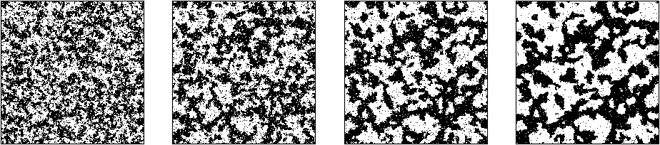
for some known, but complicated function $f$ . Even if we cannot find an analytic expression for this, we can try to approximate it. Your first idea might be “Riemann sums”, but it turns out that this is not a good idea, as our function lives in the space of all weights which has a very high dimension. Instead, we will use an approach called Monte Carlo integration where we represent the integral as an expectation value, draw a sample and approximate the expectation value by the sample average. This is where stochastical methods like Markov chains will come into play. And finally we will see that the behaviour of our network during training has some striking analogies with the behaviour of certain physical systems like solids exposed to a magnetic field at low temperatures, which are described by a model called the Ising model, and learn how techniques that physicists have developed for this type of problems apply to neuronal networks.

That is it for today – I hope I could give you a rough idea of what is ahead of us. At least I hope that you start to be curious how all this works out – so looking forward to the next post where I will start with some background from physics.

Keys in the bitcoin network: the public key

In my last post, we have looked in some detail at the private key – how it is generated and how it can be decoded and stored. Let us now do the same with the public key.

Recall that a public key is simply a point on the elliptic curve SECP256K1 that is used by the underlying ECDSA algorithm – in fact it is obtained by multiplying the generator point on the curve by our private key. As any point on the curve, it therefore has an x-coordinate and a y-coordinate, both being 32 bytes unsigned integers. So one way to encode the public key would be as follows.

take the x-coordinate as a point, represented by an integer smaller than p
convert this into a 32 byte hexadecimal string, using for instance big endian encoding
do the same for the y-coordinate
and concatenate these two strings to obtain a single 64 byte hexadecimal string

This encoding is simple, but it has a drawback. Remember that we encode not just a random pair of integers, but a point on the curve, so the x-coordinate and y-coordinate are related by the curve equation

$y^2 = x^3 + ax + b$

Thus given x, we almost know y – we know the square of y modulo p, and there can be at most two different roots of this equation. So we could reconstruct y if we have x and an additional bit that tells us which of the two solutions we need.

Let us now assume that p is odd. If y is a solution of the equation for a given value of x, then p – y (which is -y modulo p) is the second solution. As p is odd, exactly one of the two numbers y and p – y is even. We can therefore use an additional bit that is equal to y modulo 2 to distinguish the two solutions. It is convention to store this bit in a full additional byte, using the value 2 if y is even and the value 3 if y is odd, so that we obtain a representation of the public key (and in fact any other point on the curve) in at most 33 bytes: at most 32 bytes for the value of the x-coordinate and the additional byte containing the value of y modulo 2. This representation is called the compressed representation (see for instance the publication of the SECG, section 2.3).

If there is a compressed representation, you might expect that there is also an uncompressed representation. This is simply the representation that we have described above, i.e. storing both x and y, with an additional twist: to be able to distinguish this from a compressed representation that always starts with 0x02 or 0x03, a leading byte with value 0x04 is added so that the total length of an uncompressed representation is at most 65 bytes. Since version 0.6.0, the bitcoin reference implementation defaults to using compressed keys (see the function CWallet::GenerateNewKey).

Let us summarize what we have learned so far in a short Python code snippet that will take a private key (stored as integer in the variable d), calculate the corresponding point on the elliptic curve SECP256K1 using the ECDSA library and create a compressed representation of the result.

#
# Determine the public key from the
# secret d
#
import ecdsa
curve = ecdsa.curves.SECP256k1
Q = d * curve.generator
#
# and assemble the compressed representation
#
x = Q.x()
y = Q.y()
pubKey = x.to_bytes(length=32, byteorder="big")
pubKey = binascii.hexlify(pubKey).decode('ascii')
if 1 == (y % 2):
    pubKey = "03" + pubKey
else:
    pubKey = "02" + pubKey
print("Compressed key:  ", pubKey)

This way of encoding a public key is in fact not specific to the bitcoin network, but a standard that is used whenever a point on an elliptic curve needs to be encoded – see for instance RFC5480 by the IETF which is part of the X.509 standard for certificates.

However, this is still a bit confusing. If you known the nuts and bolts of the bitcoin protocol a bit, you will have seen that participants publish something that is called an address which is a string similar to

mx5zVKcjohqsu4G8KJ83esVxN52XiMvGTY

That does not look at all like a compressed or uncompressed public key. We are missing something.

The answer is that an address is in fact not a public key, but it is derived from a public key. More precisely, it is an encoded version of a hash value of the public key. So given the address, it is easy to verify that this address belongs to a certain public key, but it is very hard to reconstruct the public key given the address.

To understand the relation between a public key and an address better, it is again time to take a look at the source code of the reference client. A good starting point is the RPC method getnewaddress. This method is defined in the file wallet/rpcwallet.cpp and creates an instance of the class CBitcoinAddress which in turn is – surprise – derived from our old friend CBase58Data. The comments are quite helpful, and it is not difficult to figure out that a bitcoin address is obtained as follows from a public key.

create a hexadecimal compressed representation of the public key
apply a double hash to turn this into a sequence of 20 bytes – first apply the hash algorithm SHA256, then RIPEMD160 (this is called a Hash160 in the bitcoin terminology as the output will have 160 bits)
add a prefix to mark this as a public key address – the prefix is again defined in chainparams.cpp and and is zero for the main network and 111 for the test networks
take the hash256 checksum and append the first four bytes
apply Base58 decoding to the result

This is already very similar to what we have seen before and can be done in a few lines of Python code.

def hash160(s):
    _sha256 = hashlib.sha256(s).digest()
    return hashlib.new("ripemd160", _sha256).digest()
#
# Apply hash160
#
keyId = hash160(bytes.fromhex(pubKey))
#
# Append prefix for regtest network
#
address = bytes([111]) + keyId
#
# Add checksum
#
chk = hash256(address)[:4]
#
# and encode
#
address = btc.utils.base58Encode(address + chk)
print("Address:         ", address)

Heureka! If we run this, we get exactly the address mx5zVKcjohqsu4G8KJ83esVxN52XiMvGTY that the bitcoin client returned when we started our little journey at the beginning of the post on private keys.

As always, the full source code is also available on GitHub repository. If you want to run the code, simply enter

$ git clone https://github.com/christianb93/bitcoin.git
$ cd bitcoin
$ python Keys.py

That was it for today. We have now covered the basics of what constitutes participants in the bitcoin network. In the next few posts in this series. we will look at the second main object in the bitcoin world – transactions. We will learn how to interpret transactions, and will eventually be able to manually create a transaction to instruct a payment, sign it, hand it over to our test network and see how it is processed.

A primer on elliptic curve cryptography: practice

In the last post, we have looked a bit at the theory behind elliptic curves. In this post, we will now see how all this works down to earth and use Python to actually run some calculations.

The first thing that we need is an explicit formula for the addition of two points on an elliptic curve. We will not derive this here, but simply give you the result – see for instance [1] for more details. Given two points $(x_1, y_1)$ and $(x_2, y_2)$ , the coordinates of their sum $(x_3, y_3)$ can be determined as follows.


inv = inv_mod_p(x2 - x1, p)
x3 = ((y2 - y1)*inv)**2 - x1 - x2
y3 = (y2 - y1)*inv*(x1 - x3) - y1

Here we assume that we have a function inv_mod that will give us the inverse modulo some prime number p which is the number of elements of our base field. Typically, this can be done using the so-called extended euclidian algorithm.

However, there are a few special cases we need to consider. This is apparent if we look at this formula in more detail – what happens if the inverse does not exist because the points $x_1$ and $x_2$ are equal?

This happens if we want to add two points that have the same x-coordinate. There are two cases we need to consider. First, the y-coordinates could be equal as well. Then we are trying to add a point to itself, and we need to apply the formula provided in [1] for that special case. Or the y-coordinate of the second point is minus the y-coordinate of the first point. Then we try to add a point to its own inverse. The result will be the neutral element of the group which is usually called the point at infinity (there is a reason for this: if we embedd the curve into a projective plane, this point will in fact be the intersection of its completion with the line at infinity in the projective plane…).

To describe points on an elliptic curve, we need both coordinates, the x and the y-coordinate. Thus it makes sense to implement a class for this purpose. Instances of this class need to store the x- and y-coordinates and – for convenience – a boolean that tells us whether a point is the point at infinity. So our full code for this class looks as follows.


class CurvePoint:

    def __init__(self, x, y, infinity = False):
        self.x = x
        self.y = y
        self.infinity = infinity

    def __add__(self, other):
        #
        # Capture trivial cases - one of the points is infinity
        #
        if self.infinity:
            return other
        if other.infinity:
            return self
        #
        # First check whether we are adding or doubling
        #
        x1 = self.x
        x2 = other.x
        y1 = self.y
        y2 = other.y
        infinity = False
        if (x1 - x2) % p == 0:
            #
            # Are we talking about doubling or addition
            # of the inverse?
            #
            if (y1 + y2) % p == 0:
                infinity = True
                x3 = 0
                y3 = 0
            else:
                inv = inv_mod_p(2*y1, p)
                x3 = (inv*(3*x1**2 + a))**2 - 2*x1
                y3 = (inv*(3*x1**2 + a))*(x1 - x3) - y1
        else:
            #
            # Standard case
            #
            inv = inv_mod_p(x2 - x1, p)
            x3 = ((y2 - y1)*inv)**2 - x1 - x2
            y3 = (y2 - y1)*inv*(x1 - x3) - y1

        return CurvePoint(x3 % p, y3 % p, infinity)

As already mentioned, that assumes that you have a function inv_mod_p in your namespace to compute the inverse modulo p. It also assumes that the variables p, a and b that describe the curve parameters are somewhere in your global namespace (of course you could introduce a class to represent a curve that stores all this, but let us keep it quick and dirty at this point).

Now having these routines, we can actually do a few example and verify that the outcome is as expected. We use a few examples with low values of p from [1] .

#
# Define curve parameters
#

p = 29
a = 4
b = 20
#
# and add a few points
#
A = CurvePoint(5,22)
B = CurvePoint(16, 27)
O = CurvePoint(0,0,infinity=True)
C = A + B
assert(C.x == 13)
assert(C.y == 6)
assert(C.infinity == False)
C = A + A
assert(C.x == 14)
assert(C.y == 6)
assert(C.infinity == False)
A = CurvePoint(17,19)
B = CurvePoint(17,10)
C = A + B
assert(C.infinity == True)
A = B + O
assert(A.x == B.x)
assert(A.y == B.y)
assert(A.infinity == B.infinity)
A = O + B
assert(A.x == B.x)
assert(A.y == B.y)
assert(A.infinity == B.infinity)

For the sake of demonstration, we have shown how to build elliptic curve arithmetic from scratch. We could now proceed to implement multiplication and the ECDS algorithm ourselves, but as so often, there is a Python library that will do this for us. Well, there is probably more than one, but I like the Python ECDSA library maintained by Brian Warner.

The most basic classes in this library are – you might have guessed that- curves and points. Curves are initialized providing the basic parameters p, a and b. Then points are created by specifying a curve and the x and y coordinates of the points. Thanks to operator overloading, points can then be added and multiplied with integers using standard syntax. Here is a code snippet that reproduces the first of our examples from above using the ECDSA library.


import ecdsa

#
# Create a curve with parameters p,a and b
# with the ECDSA library
#
curve = ecdsa.ellipticcurve.CurveFp(p,a,b)
#
# Define two points and add them
#
A = ecdsa.ellipticcurve.Point(curve, 5, 22)
B = ecdsa.ellipticcurve.Point(curve, 16, 27)
C = A + B
assert(C.x() == 13)
assert(C.y() == 6)
assert(C != ecdsa.ellipticcurve.INFINITY)

Very easy – and very useful. And of course reassuring to see that we get the same result than our hand-crafted code for the arithmetic above gave us.

But this is not yet all, the library can of course do much more. Let us use it to create a signature. For that purpose, we obviously need a reasonable large value for the prime p, otherwise we could easily use a brute-force attack to determine our private key from the public key. In my previous post on the theoretical foundations, I have already mentioned the papers published by the SECG, the Standards for efficient cryptography group. This group has published some standard curves that we can use. One of them is the curve SECP256K1 which is a curve over a prime field $F_p$ with

$p = 2^{256} - 2^{32} - 2^{9} - 2^{8} - 2^{7}-2^{6} - 2^{4} - 1 = 115792089237316195423570985008687907853269984665640564039457584007908834671663$

This curve is the curve which is used by the bitcoin protocol. As many other standardized curves, it is hard-coded in the ECDSA library. To get it, use the following code.


#
# Get the standard curve SECP256K1
# and its parameters
#
curve = ecdsa.curves.SECP256k1
G = curve.generator
p = curve.curve.p()
a = curve.curve.a()
b = curve.curve.b()
n = G.order()

Let us now apply what we have learned about signatures. First, we need a private key and a public key determined from it. Thus we pick a random number that will be our secret and multiply the generator of the curve by it to get our public key.

#
# Determine a private key and a public key
#
d = ecdsa.util.randrange(n-1)
Q = d*G
pKey = ecdsa.ecdsa.Public_key(G, Q)
sKey = ecdsa.ecdsa.Private_key(pKey, d)

Next we need a hash value that we will sign. Usually, we would derive this value from a message using some cryptographic hash function like SHA256, but we will simply simulate this by drawing a random number h. We can then use the method sign of the ECDSA private key object to create a signature. This will return a signature object from which we can retrieve the values r and s.

h = ecdsa.util.randrange(n-1)
k = ecdsa.util.randrange(n-1)
signature = sKey.sign(h, k)
r = signature.r
s = signature.s

Let us verify that the algorithm really works as described the previous post. So we first need to multiply our randomly chosen integer k with the generator of the curve, the number r should then be the x-coordinate of this point. We then invert k modulo n and multiply the result by h + dr. This should give us s.

_r = (k*G).x() % n
assert(_r == r)

w = inv_mod_p(k, n)
_s = ((h+d*r)*w) % n
assert(_s == s)

If you run this code, you will hopefully see that the assertions pass. Our code works, and produces the same result as the ECDSA library. That is already reassuring. Having gone so far, we can now of course also verify the signature – again we do this once using the ECDSA library and once using our own code.

#
# Now we manually verify the signature
#
w = inv_mod_p(s, n)
assert(1 == (w*s % n))
u1 = w * h % n
u2 = w * r % n
X = u1*G + u2*Q
assert(X.x() == r)

#
# Finally we verify the signature using the
# lib
#
assert(pKey.verifies(h, signature) == True)

That is it for today. We have seen how elliptic curves can be used in practice to create and verify digital signatures and have looked at the ECDSA library that offers ready made functions for that purpose. The full source code can by downloaded from GitHub.

In my next post, I will look at the way how private and public ECDSA keys appear in the bitcoin protocol. If you want to learn more and play around a bit with elliptic curves in the meantime, I recommend the online tool [2]. You might also want to take a look at Andrea Corbellinis excellent post on elliptic curve cryptography.

1. D. Hankerson, A. Menezes, S. Vanstone,
Guide to elliptic curve cryptography, Springer, New York 2004
2. Elliptic curve point addition online tool at https://cdn.rawgit.com/andreacorbellini/ecc/920b29a/interactive/modk-add.html

A primer on elliptic curve cryptography: theory

Strong cryptography is at the heart of the blockchain and many other modern technologies, so it does not hurt to get familiar with the basics. In this post I will explain the foundations of one very commonly used algorithm called elliptic curve digital signature. This post will be a bit lengthy and theoretical but do not worry – we will see how all this works in practice in the next post.

First we need to understand what private and public keys are. At the end of the day, cryptography is about encoding and decoding messages. Suppose, for instance, that two parties (which we will call Alice and Bob to follow the usual naming conventions) want to exchange information, but expect that a third party is able to obtain a copy of every message that they send forth and back, for instance because Alice and Bob communicate over the internet and a third party could control some of the routers sitting between them (yes, we all know this is not just theory…).

One approach that Alice and Bob could use is as follows. In a first step, they both agree on a key. This could be a key phrase or some other sequence of bytes, depending on the exact algorithm they use. To send a message to Bob, Alice would then take the message $m$ and encrypt it, i.e. apply a function $f_k$ that depends on the key $k$ to obtain an encrypted message $e = f_k(m)$ .

Alice would then send the encrypted message to Bob. Bob would apply a second function $g_k$ to the received message to decrypt it again. If $f$ and $g$ are chosen properly, then they will be inverses of each other, i.e.

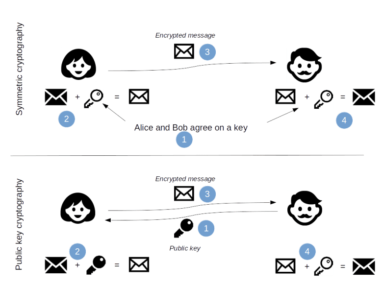
$m=g_k(f_k(m))$

Therefore Bob will be able to obtain the original message from the key and the encrypted message. The algorithm is secure if it is virtually impossible to derive the original message from the encrypted message without knowing the key.

This class of algorithms is called symmetric because both parties, Alice and Bob, use the same key, i.e. the same key is used to encrypt a message and to decrypt it again. Unfortunately, there is an obvious challenge when using this in practice: Alice and Bob need to exchange the key and therefore need a separate secure communication channel. In a peer-to-peer network like the blockchain where the nodes can only communicate via the unsecure public internet, this is virtually impossible, and a different approach is needed.

Asymmetric algorithms and public key cryptography are designed to overcome exactly this difficulty. These algorithms uses keys that come in pairs. Every key pair consists of a public key and a private key. As the naming suggests, the public key is intended to be shared, while the private key needs to be kept secret at all times. When Alice wants to send a message to Bob, she will first need to retrieve Bobs public key. Bob could for instance publish his key on a webpage or add it to the signature of an e-mail. Alice would then encrypt the message using the public key. When Bob receives the encrypted message, he uses his private key to decrypt the message again.Knowing the public key and the encrypted message is not sufficient to perform the encryption step, the private key is needed to do this. As only Bob has access to his private key, only he can read a message that has been encrypted with his public key, even though his public key is freely available and known to an attacker.

PublicKeyCryptography

Public key cryptography relies on a mathematical operation that is easy to perform in one direction, but virtually impossible in the other direction. A classical example is the factorization of large numbers. Whereas it is easy to multiply two large prime numbers $p$ and $q$ to obtain their product $n=pq$ , it requires a lot of computing power to execute the reverse operation, i.e. to determine $p$ and $q$ from $n$ . The well known RSA algorithm is based on this.

Other algorithms with this property are certain operations in properly chosen finite groups. Recall that a group is a mathematical structure in which elements can be added and subtracted such that the usual rules like associativity that we are used to from the addition of ordinary numbers apply. In particular, given a group $g \in G$ as well as an integer $k$ , we can form the product $kg$ which is obtained by adding performing k additions.

$kg = g + \cdots + g$

In some groups, the result of this operation can easily be calculated, but given $kg$ and $g$ , it is very difficult to determine $k$ . This property can be exploited to design cryptographic algorithms, as we will see in a few minutes.

One large class of finite groups with this property are elliptic curves over finite fields. Suppose that we are given some finite field $K$ (most of the time, $K$ is the prime field $F_p$ for some prime number $p$ ). Let us also assume that the characteristic of $K$ is odd. For our purposes, an elliptic curve over $K$ is the set of points $(x,y)$ that obeys an equation of the form

$y^2 = x^3 + ax + b$

with constants $a,b$ .

Finite fields are a bit difficult to visualize. To get an idea how an elliptic curve looks like, let us take a look at an example over the reals.

SECP256K1

The curve displayed here has the parameters $a=0$ and $b=7$ and features a prominent role in the bitcoin protocol (this curve over a certain finite field is known as SECP256K1, more on this in a later post). The blue line visualizes all pairs $(x,y)$ on the curve. This picture also demonstrates the reason why elliptic curves are so useful for our purposes – points on the curve can be added, and in fact the set of points on a curve forms an abelian group.

To see how the addition works, look at the points marked as A and B in the picture above. To add these points, draw a line through A and B. This line will (ignoring a few special cases and multiplicities for the time being) intersect the curve in exactly one other point, called C in this example. Then reflect on the x-axis to arrive at the point which has the same x-coordinate as C, but minus its y-coordinate. This point is, by definition, the sum of A and B.

If you have a bit of a background in algebraic geometry and that rings a bell, you are right – it has to do with divisors. In fact, the set of points on an elliptic curve is in a one-to-one correspondence with a subgroup of the divisor class group, and the group structure inherited by this relation is the one that I have just described. See [1] for more details.

So now we have a finite abelian group (remember that in reality, we do not do this over the reals but over some finite field) – what can we do with it? To illustrate this, let us describe one application to cryptography called elliptic curve digital signature algorithm (ECDSA). A digital signature is like a watermark that you add to a message to allow others to verify that you have seen and approved the message and that the message has not been altered in transit. Again, most digital signatures involve public and private key pairs. When Alice wants to sign a message $m$ , she uses her private key to encode her message and obtains a signature $s$ . She then sends that signature along with the original message and her public key to Bob. Using that information, Bob can verify the signature to confirm that it has been created using the private key that belongs to the public key and that the message that he has received is identical to the message that Alice has signed. Assuming that only Alice has access to the private key, he can then deduce that Alice has actually composed and approved the message. In practice, it is not the actual message that is signed, but a hash value of the message to keep the signature short.

Let us see how this works (in addition, [2] is a readable and valuable resource for some of the details). Suppose Alice wants to sign a message $m$ . The first thing she will do is to agree with Bob on some set of elliptic curve parameters, i.e. a finite field, the parameters $a$ and $b$ and some point $G$ on the curve called the generator. In [2], a few standard sets have been defined and published, among them the standard SECP256K1, on which Alice and Bob could agree. That information is public and does not need to be protected.

Next, Alice will pick a secret or private key. In our case, this is simply a number $d$ between zero and the order $n$ of the point $G$ . Alice will then determine a public key

$Q = dG$

which is simply a point on the curve. That key can be freely published – as we have mentioned before, it is computationally very hard to determine the secret $d$ from that information.

All this only needs to be done once. Now comes the part that is specific to the message. First, Alice create a hash value of the message by applying a hash function:

$h = H(m)$

The hash function needs to be chosen such that the resulting hash value can be interpreted as a number between zero and $n - 1$ . Next Alice picks a random number $k$ between one and $n - 1$ and determines the coordinates of the point $kG$ . Let $r$ denote the x-coordinate of this point. Then Alice determines

$s = k^{-1}(h + dr) \mod n$

where the inverse is taken modulo n. The signature that Alice will publish along with the original message is then the pair $(r,s)$ .

When Bob wants to verify the signature, he would then again compute $h = H(m)$ and determine the point

$X = s^{-1} hG + s^{-1} rQ$

on the curve. Let us do a short calculation to see what the expected outcome is. First,

$X = s^{-1}(h + rd) G$

Now by the choice of $s$ , we also have

$s^{-1} = k(h+dr)^{-1} \mod n$

Therefore

$s^{-1}(h+dr) = k \mod n$

As $n$ is the order of $G$ , this implies that

$X = kG$

Thus we expect that the x-coordinate of the newly computed point $X$ is equal to the x-coordinate of $kG$ which Alice has published as $r$ . If Bob makes this comparison and arrives at this result, he can be almost sure that someone who has access to the private key has signed the message and that the message has not been altered since then.

Note that, if we knew the signature and $k$ , we could compute $h + dr$ and therefore the secret $d$ . It is therefore extremely important to treat the number $k$ with care – use a strong random number generator to obtain it, do not reuse it for further messages and delete it immediately after using it.

We have now seen how arithmetic on an elliptic curve can be used to design a secure and reliable digital signature. I admit that this was a bit theoretical, but now comes the fun part – in the next post we will see how this can be done in Python and code a few examples. Stay tuned…

1. R.Hartshorne, Algebraic Geometry, Springer, New York 1997, example 6.10.2
2. Standards for efficient cryptography 1 and 2 (SEC1, SEC2), SECG Group, available online at http://www.secg.org